Transitional Bass Reflex Alignments

This is the fifth article in my series about the invention, concept, and historical perspective of loudspeaker bass reflex alignments. In the May issue, we started with “Computation of Bass Reflex Alignments,” in which I presented, among other classical alignments, the B4 alignment, then in the June issue, I presented the LR4 alignment. These were followed with the IB4 vented alignment article in the July issue, and most recently, the CD4 vented alignment in the August issue.
 
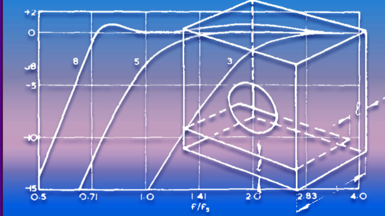
Notably, R. M. Golden and J. F. Kaiser [1] described the roots of normalized Butterworth and Bessel-Thomson low-pass transfer functions, from which Richard Small [2] derived the polynomial coefficients of the fourth-order high-pass Bessel alignment. Golden and Kaiser also described a transitional filter design where a chosen balance between the two is realized.

The concept of transitional alignments is helpful in bridging between alignments, not least discrete alignments, for which we can obtain a continuous family of alignments, which could prove to be a practical concept worth exploring. Transitioning means that you no longer target strongly, for example, either the maximally flat frequency response or the maximally flat group delay but wish to compromise between the two. However, it seems that the idea of transitional alignments has not been investigated in literature related to loudspeakers.

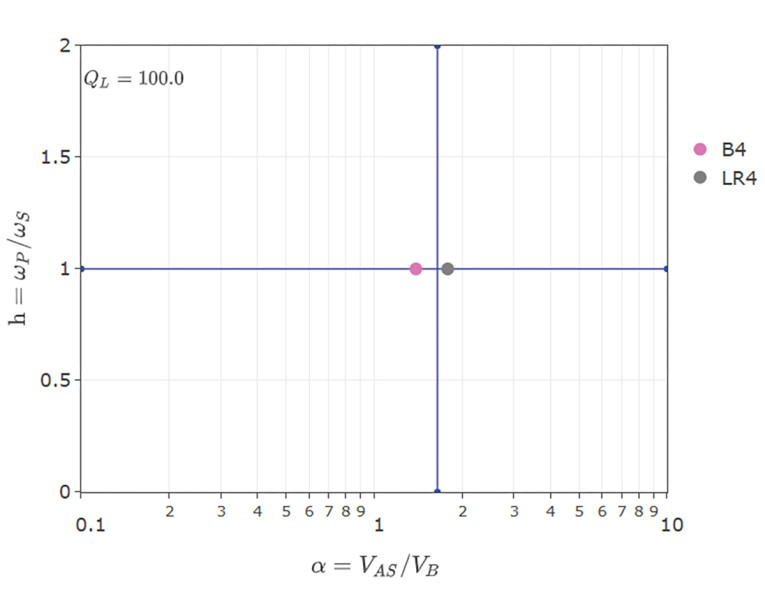
In this article I wish to present the transitional alignment between Butterworth B4 and Linkwitz-Riley LR4. Many other transitional alignments are possible. For any given driver Qt value, it is possible to transition between alignment options, by selecting an alpha and h value between the two alignment options. A graphical view can be created if you lay out the bass reflex alpha and h parameters in a 2D chart.

Bessel-Butterworth
Before we dive into the primary purpose of this article, let us look at the Golden and Kaiser approach to transitioning between normalized Bessel and Butterworth (low-pass) transfer functions.

The poles of the response function are defined in polar coordinates:
where:

t = transition factor

r_n = modulus of the nth pole

r_BL_n = modulus of the nth Bessel filter pole

Theta_n = phase angle of the nth pole

Theta_B_n = phase angle of the nth pole of the Butterworth filter

Theta_BL_n = phase angle of the nth pole of the Bessel filter

We conclude that transitioning is a simple study of the pole location(s) and some interpolation scheme. When t = 0, we have transitioned entirely to the Butterworth response, whereas t = 1 gives the Bessel response. For the calculation of r_n, there is no need to include the Butterworth response because the modulus of all poles is 1 (they are located on the unit circle).

Mathematical Description of B4-LR4 Transition
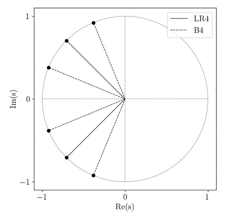
Studying the poles of the polynomial transfer function in the s-plane, we know that the LR4 response function has two double poles, located at theta = ±3/4 pi (±135 degrees), whereas the B4 response function has equally spaced poles, located at theta = 5/8 pi, 7/8 pi, 9/8 pi, and 11/8 pi (45 degrees apart); see Figure 1.
 
We can write a one-parameter family of alignments that contains both B4 and LR4 as specific cases. Consider:
where epsilon is an angle for which 0 <= epsilon <= pi/8. Geometrically, epsilon is an angle for which the four distinct poles of the response function lie on the unit circle at s = e(i theta) at theta = 3/4 pi ±epsilon and theta = -3/4 pi ±epsilon. We can see that for epsilon = 0, we have the LR4 response function, and for epsilon = pi/8, we have the B4 response function.

It is a characteristic of the BB4 (LR4) and B4 alignments that they are “symmetric,” by which I mean a1 = a3, which also implies h = a3/a1 = 1 (this equation is correct in general for lossless alignments, but for symmetric alignments with a3 = a1, it also works in the lossy case). Examples of non-symmetric alignment, which is not treated in this article, are, for example, the Bessel alignment (BL4), the Sub-Chebychev alignment (SC4), and the Quasi Third-Order Butterworth alignment (QB3, including IB4).

The Calculation Including Leakage Loss
For a given driver Qt value, we have:
Qt = 1./(√(a1*a3) - 1/Ql). We may isolate a1 = a3 based on user-specified Qt and Ql values. This works provided that the Qt value is somewhere between the LR4 and B4 limits; for Ql = 100, we get 0.355 < Qt < 0.384. The following Scilab code shows how to transition between B4 and LR4, given a driver Qt value and system leakage Ql value:
where we take advantage of the fact that h = 1 for both the LR4 and the B4, as well as any transitional alignment we choose between the two, and simplify the expressions.

Graphical View
As mentioned previously, we may show alpha and h on a 2D chart as seen in Figure 2. For Figure 2, I have plotted the B4 alignment as well as the LR4 (BB4) alignment, as calculated with a driver Qt-value of 0.37 (i.e., with some degree of misalignment). The presented transitional alignment, which is computed for Qt = 0.37 in the above code snippet, is marked with the blue cross. It is near the LR4 alignment, moving toward the B4 alignment. The SEAS H1571-08 (U18RNX/P) driver with Qt = 0.37 [3] matched our desired model computation and was loaded into Speakerbench to generate Figure 2.
 
Summary
I have shown how you can transition between alignments, mathematically working with the poles of the transfer function, and how these transitions can be laid out in a 2D alignment chart located somewhere between two (or several) known alignments, such that you can work with transitions in a graphical way, although not as mathematically precise a method as calculation of the pole shift.

Here I briefly mentioned the Bessel-Butterworth transitional alignment, as discussed by Golden and Kaiser. We presented how to compute the LR4-B4 transitional alignment. Another transitional alignment, just as an example, could be for drivers in the Qt range of approximately 0.34 to 0.36 (depending on Ql), for which the IB4-LR4 transitional alignment could be interesting to explore as a compromise. In the Speakerbench [4] alignment chart, it is straightforward to select a point and evaluate the alignment regarding frequency response, group delay, and other relevant performance measures.

Speakerbench currently does not list any transitional alignments explicitly in the BOX app; instead, you must aim with your pointer and click somewhere in-between the known alignments, and then in the Settings tab, you click the APPLY button to transfer the alpha and h values into a Vb and fp value for box simulation.

With the calculated transition from LR4 to B4, we have obtained a subtle improvement over continuing with the Boombox alignment. For drivers with Qt values above the LR4-Qt, the Boombox alignment will have a (small) peak in its frequency response before roll-off. By transitioning towards the B4 alignment, we avoid this peak, and the frequency response remains monotonic. VC

Author Acknowledgment: Thank you to Jeff Candy, who came up with the idea of a transitional alignment between LR4 and B4, and he helped with the derivation of the algorithms implemented into the Alignment Chart of the Speakerbench web application.


References
[1] R. M. Golden and J. F. Kaiser, “Root and Delay Parameters for Normalized Bessel and Butterworth Low-Pass Transfer Functions,” IEEE Transactions on Speech and Audio Processing, Volume AU-19, March 1971.
[2] R. H. Small, “Vented-Box Loudspeaker Systems Part IV: Appendices, Journal of the Audio Engineering Society (JAES), Volume 21, Issue 8 pp. 635-639, Oct. 1973. https://www.aes.org/e-lib/browse.cfm?elib=1941
[3] Simulation of the SEAS U18RNX/P datasheet, https://loudspeakerdatabase.com/SEAS/H1571-08_U18RNX-P
[4] Speakerbench, https://speakerbench.com


This article was originally published in Voice Coil, September 2024