The concept of loudspeaker bass reflex alignments was introduced by A. N. Thiele in 1961 and evolved through the 1970s and 1980s. Through the heydays, these alignments were communicated to the DIY community with tables where QL (= Ql), QT (= Qt), h, alpha, and f3/fs is presented as a table in an easily digestible way. A great reference for these alignment tables is found in an article series in Speaker Builder Magazine [1] by Robert Bullock; later, the same material was published in a book titled Bullock on Boxes.
These tables are not an ideal approach for computerized development tools. Sometimes the tables were just implemented directly, and either you would have to choose a fitting alignment from the table or possibly the software, which includes some interpolation scheme to allow the user to specify Ql and possibly Qt with different values.
As far as we know, mathematical presentation of the various alignments does not exist in a single source and consolidated form. Each software developer who wants to implement the alignments with user-specified (arbitrary) Ql-value would have to look into the scientific articles and develop the mathematical expression for the alignments.
In this article, we wish to fill the gap and present the math for a selection of well-known alignments. The math sometimes requires an iterative process, an optimization or root-finding process, and is in the form of an algorithm presented as a Scilab code snippet.
It is interesting that the only input parameter needed for the calculation of an alignment is the driver’s Qt-value. The output is two normalized parameters named alpha and h, where alpha is the ratio of driver Vas over the box volume (Vas/Vb) and h is the ratio of port tuning frequency versus the driver’s resonant frequency (fp/fs).
In other words, to convert these normalized parameters, you need to know Vas and fs for the driver. That is quite elegant because this is all you need to (approximately) reproduce a desired filter response function in a bass reflex design. This article builds on the presentation by Richard H. Small [2,3], and it could be a good idea to have those articles at hand while reading this article.
Intro to Scilab
Scilab is free, open-source software available at www.scilab.org. Scilab is similar to MATLAB but not exactly code compatible. If you are familiar with MATLAB, it should be easy to adapt the code. Scilab has an Integrated Development Environment (IDE) with a nice Graphical User Interface (GUI) similar to an older version of MATLAB and a built-in code editor (SciNotes), where you can dump the presented code from this article and execute it (push the PLAY button). Alternatively, you can copy-paste the code directly into the Scilab console window, and it will execute on the fly. Scilab code has a natural mathematical look and feel (similar to MATLAB), which makes it easy to translate into other programming languages, even for someone who isn’t familiar with Scilab. Scilab can run on Microsoft Windows, MacOS, and GNU/Linux machines.
We have chosen not to use Python code in spite of Python being one of the most popular programming languages today (we use it ourselves) because it is under continuous development, which means code may become depreciated over time. Besides, Python code would require additional libraries like Numpy and Scipy; each code snippet would require some initialization header; and Python doesn’t have a nice GUI (IDLE looks scary). Anyway, if you have some degree of Python wizardry, the presented Scilab code should translate easily.
Overview
Table 1 depicts the alignments that we are computing in this article, in order of appearance (Qt range is valid with leakage loss Ql = 10). The alignments in Table 1 are considered classical alignments. These alignments are all defined by a high-pass response function, which in general is described as a normalized fourth-order polynomial:
G(s) = s4 / (s4 + a1 s3 + a2 s2 + a3 s + 1)
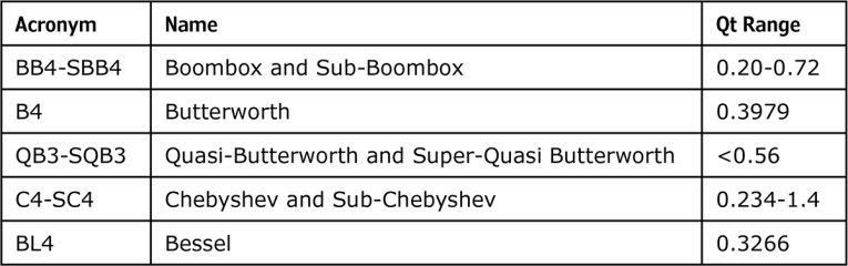
where a1, a2, and a3 are polynomial coefficients that define the response (i.e., the alignments in Table 1 can be defined with three coefficients). Whenever we calculate the bass reflex parameters alpha and h, we attempt to match the response function. The relationship between the coefficients and the bass reflex parameters is given by information from Small [2, Eqs. 22-24].
The fourth-order polynomial in the denominator has four roots (i.e., when s = a root value, the result is zero). Since these zeros are in the denominator, we divide by zero, and the result is infinity. Therefore, these points are called poles. For further illustration, these are sometimes plotted in a pole-zero plot. In summary: To identify the poles, we look for the zeros in the denominator. I am mentioning this because, in this article, we will from time to time talk about the poles and their location in the s-plane.
Boombox (BB4)
First, we look at the Boombox alignment by W. John Hoge [4]. The reason we chose this one as a starting point is because it is incredibly simple. The simplicity stems from the definition that the fourth-order polynomial, which describes the response function, is defined as two identical cascaded second-order polynomials. This reduces the math to a one-parameter family of responses, and it is equally as simple as calculating a closed box. The response function:
G(s) = s^4 / ( (s^2 + 2 zeta s + 1)^2 )
where zeta is the damping ratio, which is a value that depends on the driver’s Qt-value. If the system is calculated as lossless, then zeta = 1/(4 * Qt). For calculation of a bass reflex box and its parameters, alpha and h, we follow the algorithm below:
Ql = 10
Qt = 0.367
h = 1
alpha = 1./4 * (1./Qt - 1./Ql).^2
Qt = 0.367
h = 1
alpha = 1./4 * (1./Qt - 1./Ql).^2
In this code, insert whatever Ql and Qt values for which you wish to compute. Scilab includes a variable browser, where you can study each of the variables. Alternatively, you can add a “disp” or “printf” statement to the code to display (print) parameters in the console window. The h output parameter is always 1 for the boombox alignment, by definition.
If you let Qt be a vector (array) of variables, example: Qt = [0.40 0.50 0.60], and possibly change Ql to match the alignment table you wish to reproduce, then you can reproduce the tables by Bullock, or a subset of the tables.
It is worth noting that if Qt = Ql, then we have a discontinuity (alpha = 0). A low Ql-value equivalent to a driver Qt value seems quite inappropriate for bass reflex, and in practice, it is reasonable to expect that Ql is always much larger than Qt.
The lowest Ql-value that Bullock [1] presents is 3, but even that is borderline exceptionally bad; meanwhile, one would be hard-pressed to find a driver with Qt = 3 (it could be reached with significant DC resistance in series with the driver, but only if the driver’s Qm-value is even higher).
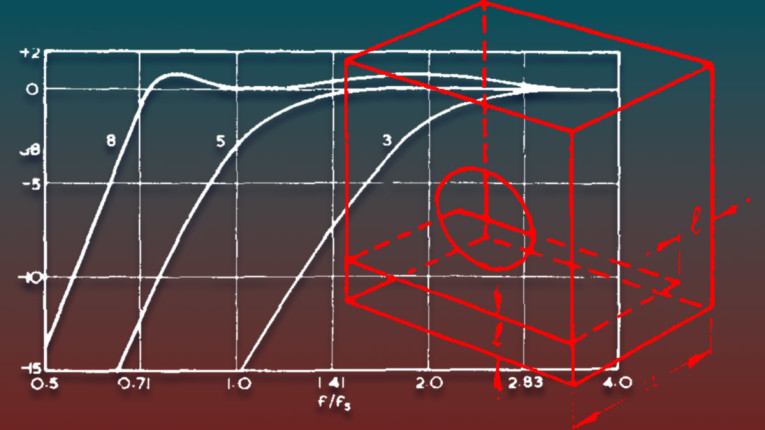
Hoge was focused on a suitable alignment for instrument loudspeakers (e.g., for electric guitars) and was seeking a better bass reflex alignment option for the high Qt-drivers of the time than the classical Chebyshev C4-alignment. Choosing to cascade two identical second-order polynomials gives double poles and therefore a nicer group delay with a reasonably fast settling time for an impulse. Unfortunately, this alignment always creates a peak before roll-off, and Hoge, who is a witty person, named it the Boombox alignment, or BB4.
Hoge only defined the BB4 alignment for driver Qt above ca. 0.37, and he identified the peak with Ql = 7 for a driver Qt = 0.72 to be around +6dB. For high Qt drivers, the peak becomes large, which you might accept in favor of the impulse stopping quicker than a similar peaky Chebyshev response.
Besides, the single peak of a BB4 alignment is easier to equalize electronically, than the ripples of a Chebyshev alignment. On the other hand, a Chebyshev alignment with similar driver Qt results in 1.3dB to 1.4dB ripple. Finally, when driver Qt is this high, one may consider a large, closed box.
Bullock realized that the equations also work well for drivers with lower Qt, and in this case, there is no peak in the frequency response. He coined the term Sub-Boombox for these alignments, or SBB4, and his tables go as low as Qt = 0.20. It is therefore reasonable to say that the BB4-SBB4 alignment works for driver Qt in the range of 0.20-0.72, although mathematically you are free to calculate outside these limits.
Butterworth (B4)
Stephen Butterworth defined the Butterworth response around 1930 as the maximally flat frequency response without a peak (or dip). Maximum flat frequency response sounds good in the ears of many engineers, and for this reason, the Butterworth responses of all orders have been a desired target for many loudspeaker designs as well as electrical filters, etc.
For bass reflex to have maximally flat response, the driver and tuning must be carefully matched, which means the Butterworth B4 alignment is a discrete alignment, and therefore Qt is not something you can set, but it is computed based on the chosen Ql-value:
Ql = [3 5 7 10 15 20 50]
Qt = 1./(1./cos(3*%pi/8)-1./Ql)
h = 1
a3 = sqrt(8)*cos(%pi/8)
alpha = sqrt(2) - (1./Ql.^2) .* (a3*Ql-1)
for i = 1:length(Ql)
printf( ..
"QL: %i QT: %.4f h: %i alpha: %.4f\n", ..
Ql(i), Qt(i), h, alpha(i))
end
Qt = 1./(1./cos(3*%pi/8)-1./Ql)
h = 1
a3 = sqrt(8)*cos(%pi/8)
alpha = sqrt(2) - (1./Ql.^2) .* (a3*Ql-1)
for i = 1:length(Ql)
printf( ..
"QL: %i QT: %.4f h: %i alpha: %.4f\n", ..
Ql(i), Qt(i), h, alpha(i))
end
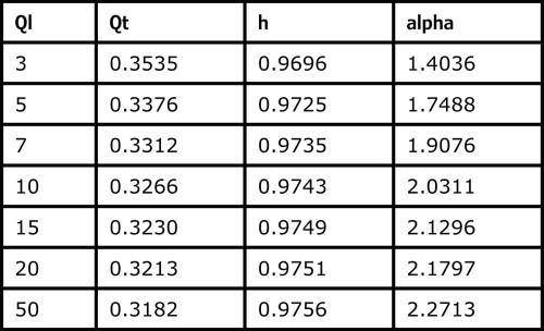
Here we have already defined the leakage Ql-value as a vector, and the printf statement at the bottom in a for-loop will reproduce and display the fourth-order Butterworth alignment table as found in Bullock’s Table XIX [1].
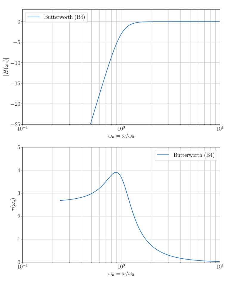
The a3-value is used as a “helper” to simplify the expression of alpha. In fact, a3 is one of the three coefficients of the (normalized) polynomial for a fourth-order Butterworth response.
If you like to condense mathematical expressions, feel free to take the expression for a3 and insert it into the equation for alpha directly. The other coefficients of a Butterworth response are: a1 = a3, and a2 = 2 + √2. With these coefficients, it is possible to calculate and plot the response function magnitude and group delay (calculated from the phase response and seen in Figure 1). Please note, once you set a finite Ql-value, then the target response function is not exactly met anymore.
Quasi-Butterworth Third-Order (QB3)
The QB3 alignment is one of the alignments invented by Thiele in his seminal two-part article series [5]. I can imagine that Thiele was interested in something Butterworth-like, but which could be applied to drivers with Qt values that did not match the discrete B4 alignment. Indeed, the QB3 works for any loudspeaker with a Qt below the B4 value (i.e., for Ql = 10), anything below 0.3979 (or ca. 0.40). He solved this by relaxing the requirement for a maximally flat response.
Therefore, this alignment is designed for returning something that resembles a third-order Butterworth response in the transition from the passband into the stopband, hence its name, QB3 (not QB4). As you go further into the stopband, the asymptotic behavior is a fourth-order response, like all fourth-order systems. In practice, Qt above 0.34 will be closer to a fourth-order response, also in the roll-off transition.
The QB3 alignment was a preferred alignment by many designers/engineers for many years because of its resemblance to the Butterworth B4 and because the box volume turns out quite small. A compact cabinet is often a desired design feature. Generally speaking, lower driver Qt results in a smaller box volume and a roll-off response closer to the third-order Butterworth response.
Bullock realized that the equations also work for drivers with higher Qt, and in this case there is a peak in the frequency response. He coined the term Super-QB3 for these alignments, or SQB3. Although named “super,” the response has a peak and isn’t super-good. Super just means “above” the Qt of a B4 alignment. With this extension, Bullock tabulated the QB3-SQB3 alignment for drivers with a Qt value as high as 0.56, which Bullock shows has a +11.6dB peak (ugh!). The crossover point that joins QB3 and SQB3 is the B4 alignment.
To find out how to relax the Butterworth conditions, we iterate over h.
Ql = 10
Qt = 0.34
h0 = 1e6 // Initialization
tol = 1e-8
q2 = Qt.^2 // A helper
e = Qt/Ql
r0 = 8*q2 * (1-q2)
h = 1./sqrt(r0)
while abs(h-h0) > tol do
h0 = h
da = 8*q2*e/h*(1+h.^2+e*h)
db = ((1+e*h).^4-1)/h.^2
r = r0+da-db
h = 1/sqrt(r)
end
alpha = -(1+h.^2)+(1+e*h).^2/(2*q2)-e*h/q2
Qt = 0.34
h0 = 1e6 // Initialization
tol = 1e-8
q2 = Qt.^2 // A helper
e = Qt/Ql
r0 = 8*q2 * (1-q2)
h = 1./sqrt(r0)
while abs(h-h0) > tol do
h0 = h
da = 8*q2*e/h*(1+h.^2+e*h)
db = ((1+e*h).^4-1)/h.^2
r = r0+da-db
h = 1/sqrt(r)
end
alpha = -(1+h.^2)+(1+e*h).^2/(2*q2)-e*h/q2
Note: The QB3 alignment is based on B4 in the way that some polynomial coefficients (A1 and A2) are kept equal to zero, but the least significant coefficient (A3) is allowed to change in a way that, depending on driver Qt, matches the amplitude of a B4 filter. In a general way, we could call this technique Amplitude Matching.
Amplitude Matching is based on the eighth-order polynomial you get when multiplying the fourth-order (normalized) response function with its complex conjugate. This produces an eighth-order polynomial, which only describes the magnitude of the response (phase information is gone). The coefficients of this eighth-order polynomial typically has capital-letters (as in A1, A2 and A3). See the Small articles [2, 3] for details.
Chebyshev (C4)
The Chebyshev alignment was first studied by F. J. van Leeuwen [6]. There are in fact two kinds, as sketched by van Leeuwen in his Figure 22 (type 1) and Figure 23 (type 2). The most commonly discussed is the type 2 kind, and it is the one Bullock has tabulated. Although it could be interesting to study Chebyshev in detail, in this article we will keep to the commonly used type 2, to replicate the tables of Bullock.
Chebyshev is defined as an equal ripple response, which at the same time implies that the response has maximum bandwidth with minimum ripple because ripple is kept within a limited band (hence ripples are kept equal).
It was Thiele who proposed to extend the calculations into the range of drivers with lower Qt and named it Sub-Chebyshev (SC4), in which case there is no ripple anymore. The crossover between C4 and SC4 is (again) the B4 alignment. Obviously, B4 was a popular target.
Back in the day, before Bullock published his findings, it was normal to consider the QB3-B4-C4 alignments as a natural, continuous, extended range of options that could be applied to a very large range of drivers, at least anything that could possibly be relevant for bass reflex designs. Bullock’s articles opened the eyes of loudspeaker designers for alternatives.
SC4 as a competitor to QB3 has a shorter settling time (better transient response), the box volume is a bit smaller (Qt range 0.3 - 0.4), the frequency response goes a bit less deep before roll-off, and in the past was typically considered less attractive to speaker designers. The SC4 resides between a QB3 and a SBB4 alignment and could in practice be an excellent compromise.
Ql = 10
Qt = 0.54
h = 0// Initialization
tol = 1e-8
e = Qt/Ql
z = 8*(1+sqrt(2))*Qt.^2
a0 = z-1
b0 = z*(sqrt(8)-1)-6
c0 = -1
x = ( -b0 + sqrt(b0.^2-4*a0*c0) ) / (2*a0)// quantify ripple
x0 = 1e6
while abs(x-x0) > tol do
x0 = x
d = (x.^2+6*x+1)/8
p = ( 1 - (1-x)/sqrt(8) ) / sqrt(d)
q = Qt.^2 * x * (4+sqrt(8)) / sqrt(d)
dp = e*(p.^2-1) / (1-e*p)
dq = 0.5 * ( -(q+2*e) + ..
sqrt((q-2*e).^2 - 4*e.^2) )
dw = q*dp + p*dq + dp*dq
a = a0 + dw
b = b0 + 6*dw
c = c0 + dw
x = (-b+sqrt(b.^2-4*a*c))/(2*a)
end // outside Qt-range, this runs
k = sqrt(x) // into negative x-values
h = q + dq
a2 = ( 1 + x*(1+sqrt(2)) ) / sqrt(d)
alpha = -(1+h.^2) - e*h/Qt.^2 + a2*h
K = 1/k.^2 - 1
// calculate ripple, just curious
dB_ripple = 10 * log10(1 + K.^4 ./ ..
(64 + 28*K + 80*K.^2 + 16*K.^3))
This algorithm has some limitations to the driver Qt value, such that if leakage Ql = 7, then driver Qt must be kept between 0.236 and 1.026 (not a difficult criteria), or if Ql = 10, then driver Qt must be kept between 0.234 and 1.416. If you neglect these limits, the algorithm might fail.
Please note that the Chebyshev alignment is an entire family where you can specify the desired ripple. The alignment tables and above algorithm always lay out the minimum amount of ripple, but let us say the driver at hand can meet, for example, 0.25dB ripple, but you don’t mind 2dB ripple, then the Chebyshev family of alignments in principle can extend the frequency response further, but the payback is even lower quality of transient response.
The flexibility stems from the mathematics that a Chebyshev alignment doesn’t have its poles on the unit circle, but on an ellipsis and the elliptical shape can be controlled. Chebyshev filters are a limit case of the Cauer Elliptic filters, which all show the equal ripple behavior.
Bessel (BL4)
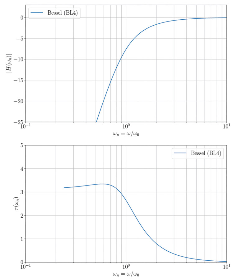
The Bessel alignment was mentioned by Small [2, 3], and he simply references Golden and Kaiser for the roots of the polynomial response function and proceeds to present the polynomial coefficients. It is a discrete alignment only realizable with a very specific driver Qt.
Ql = 10
// The polynomial coefficients:
a1 = 3.20108
a2 = 4.39155
a3 = 3.12394
// Lossless Qt0 = 1./sqrt(a1*a3)
// = ca. 1./ sqrt(10)
Qt = 1./(sqrt(a1*a3) - 1/Ql)
A = a1/a3
e = Qt./Ql
h = (1 - A * e)./(A - e)
alpha = a2*h - h.^2 - 1 - ..
(a3*sqrt(h)*Ql - 1)./Ql.^2
// The polynomial coefficients:
a1 = 3.20108
a2 = 4.39155
a3 = 3.12394
// Lossless Qt0 = 1./sqrt(a1*a3)
// = ca. 1./ sqrt(10)
Qt = 1./(sqrt(a1*a3) - 1/Ql)
A = a1/a3
e = Qt./Ql
h = (1 - A * e)./(A - e)
alpha = a2*h - h.^2 - 1 - ..
(a3*sqrt(h)*Ql - 1)./Ql.^2
Table 2 shows the alignment table for the Bessel alignment, like it is found in Bullock [1] Table XIX. Challenge to the reader: Download Scilab and modify the above code, defining Ql as a vector, such that it prints the table. Hint: Remember to use a dot when element-wise operation is required.
However, these attributes are for low-pass Bessel filters, it is not necessarily true for the derived high-pass Bessel function used for loudspeaker alignments. Maximally flat group delay is not the same as minimum group delay. The magnitude response and group delay is plotted in Figure 2. Note: In principle we have a discontinuity at around Ql = 1/√10, so one must keep Ql > 0.317 (such a low Ql would be absurd anyway).
Summary
Generally speaking, to define these alignments mathematically requires some work with various sources, and we hope the reader appreciates that they are now collected here in this article and presented in a consistent and uniform way.
The two discrete alignments, B4 and BL4, might seem a bit tricky to reach since they require a driver with a specific Qt value. You will never get this 100% correct, but with a leakage Ql-value, you are also not 100% there, so one may allow some degree of misalignment, say, for example, a 5% error in Qt, and you should still be doing OK.
One of the reasons to develop the theory and define certain alignments, in particular the discrete alignments, is that they create fix-points in the universe. These discrete alignments all have special meanings, like maximum bandwidth, most linear group delay, or possibly some specific location of the poles in the s-plane that facilitate certain characteristics. These fix-points are useful when navigating in the 2D space represented by alpha and h.
Classical Thiele-Small theory prescribes that one sets Ql = 7 or 10 or some other arbitrary number. The value is not representative of the true leakage loss of the system but a mix of various loss contributions. Therefore, the practice of setting Ql to some low value is questionable, but in this tutorial article, we keep Ql as prescribed by the theory. Setting Ql to some low value will result in a smaller alpha-value, by which you end up calculating a larger box, and it seems like this has been chosen as a way to retrieve a conservative estimate, such that the speaker builder would end up with a box large enough and, in the process, not falling short in box volume and having to rebuild new and larger boxes. This implies that you’re welcome to choose a different value for Ql.
I wonder if the fear of building a too-small box belongs in the past. The reasons were: 1) the builder relied on manufacturer specifications, which might contain errors; 2) the builder measured the driver’s Thiele-Small parameters, but the process was error-prone; 3) manufacturing tolerances in production. Today, manufacturer specs are typically correct because modern testing and fabricating datasheets with computers ensure they are error-free. Manufacturing tolerances have been mitigated and the dominant factor is the suspension stiffness, which is not as critical as other factors. VC
Author Acknowledgment: Thank you to Jeff Candy, who helped with the derivation of these algorithms, as implemented into the Alignment Chart of the Speakerbench [7] web application.
References
[1] R. M. Bullock, III, “Thiele, Small and Vented Loudspeaker Design, Part I - IV,” Speaker Builder Magazine, 1980-1981. Part 4 in Number 3 (Jul./Aug./Sep.) 1981, pp. 18-27.
[2] R. Small, “Vented-Box Loudspeaker Systems - Part I: Small-Signal Analysis,” Journal of the Audio Engineering Society, Vol. 21 Issue 5, pp. 363-372; June 1973.
[3] R. Small, “Vented-Box Loudspeaker Systems - Part IV: Appendices,” Journal of the Audio Engineering Society, Vol. 21 Issue 8 pp. 635-639; October 1973.
[4] W.J.J. Hoge, ”A New Set of Vented Loudspeaker Alignments,“ Journal of the Audio Engineering Society, Vol. 25, Issue 6, pp. 391-393; June 1977.
[5] A. Neville Thiele, “Loudspeakers in Vented Boxes: Part 1 - 2,” Proc. IREE (Australia), Volume 22 (1961). Republished in the Journal of the Audio Engineering Society, Vol. 19, May and June 1971.
[6] F. J. van Leeuwen, “De Basreflexstraler in de akoestiek,” Tijdschrift van het Nederlands Radiogenootschap, Vol. 21 No. 5, September 1956.
[7] Speakerbench, https://speakerbench.com
This article was originally published in Voice Coil, May 2024