Voice Coil Focus: Quasi-Alignment Families

This article is another great contribution by Claus Futtrup, this time with direct support from Jeff Candy, the two creators of Speakerbench, the free to use web-based application for low-frequency analysis and design of loudspeakers. Another follow-up article for the “Computation of Bass Reflex Alignments” article series that was published in Voice Coil’s May through October 2024 issues, this time, the authors discuss the important Quasi-Alignment Families where the fundamental idea is trying to approach a roll-off similar to the Butterworth B4 alignment (a maximally flat response) but compatible with real systems for which the driver Qt will not allow a true B4 alignment. Something that Neville Thiele defined earlier as a QB3, or Quasi Butterworth alignment.
 
A.N. Thiele defined the QB3 (the Quasi Butterworth) alignment in his seminal article series, “Loudspeakers in Vented Boxes,” Part 1 and Part 2 [1]. The fundamental idea is that you desire a roll-off similar to the Butterworth B4 alignment (a maximally flat response) but compatible with real systems for which the driver Qt will not allow a true B4 alignment (because B4 is a discrete alignment). Note that QB3 is a family of alignments, with B4 as a limiting case, where the requirements for the polynomial response are relaxed. In this article, we describe how this is executed in practice.

Basic Theory
Vented alignments are particular types of fourth-order high-pass filters. Following Richard Small [2], we can write the normalized response function as:

G(s) = s4 / (s4 + a1 * s3 + a2 * s2 + a3 * s + 1)

where s = j * w / w_0 is the dimensionless complex frequency variable normalized to w_0 = √(w_B * w_S). Once we set s to an imaginary number, we investigate the true normalized frequency response. The squared modulus of the above equation is calculated as G(s) * G(-s) because the coefficients are real, and gives the following real expression for the frequency magnitude response (squared):

│G(j*w)│2 = w8 / (w8 + A1 * w6 + A2 * w4 + A3 * w2 + 1)

It is possible to replace x = w2 and keep analyzing a fourth-order function. It seems this is a favorite method for Thiele to explore the characteristic response. To relax the response requirements for a B4 and arrive at the QB3 alignments, Thiele chose to relax the A3 coefficient since this term is the least significant of the three in the passband (i.e., the response “error” is weighted toward the stopband). The presentation by Small [2] is clearer, and you will find the squared modulus expression in his Equation 58.

Small then continues by defining the relationship with the normalized transfer function:

A1 = a12 - 2 * a2

A2 = a22 + 2 - 2 * a1 * a3

A3 = a32 - 2 * a2

Furthermore, in Small’s Equations 22-24 [3], he writes the lossy polynomial filter coefficients as:

a1 = (Ql + h * Qt) / (√(h) * Ql * Qt)

a2 = (h + (alpha + 1 + h2) * Ql * Qt) / (h * Ql * Qt)

a3 = (h * Ql + Qt) / (√(h) * Ql * Qt)

where Ql is the leakage loss Q of the box and Qt is the total Q of the driver. Here h = w_B / w_S is the system tuning ratio, and alpha (α) = Vas / Vb is the ratio of the compliance volume to the box volume. We remark that the coefficients are approximate and neglect myriad other terms, which appear in a more comprehensive model of a vented box. These missing terms would represent more complex losses in the box and in the driver suspension system, driver inductance and semi-inductance, and so on. In the definition of w_0, w_S is the driver resonant frequency and w_B is the vent resonant frequency. This normalization is equivalent to setting T_0 = 1 in Small’s expressions.

We summarize the values for the A coefficients, as well as Qt for the lossless case:
 

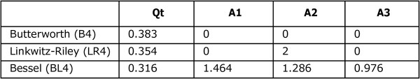
It can be observed that the normalized fourth-order Butterworth filter has A1 = 0, A2 = 0, and A3 = 0, which gives the mathematical feature of maximal flatness in the frequency response. Since these respective alignments are possible only for a single value of Qt, a procedure is required to extend (or approximate) them for a continuous range of Qt.

Generalized Quasi-Alignments
In a design process based on alignments, we consider Ql and Qt as given inputs and alpha and h as output parameters to be computed by the alignment. Since we have two free parameters, it follows that we can specify only two of the three values A1, A2, and A3. The approach taken is to relax (i.e., ignore) the condition on A3; that is, we match the behavior in the passband (A1) and midband (A2) but not the stopband (A3). This is described in great detail for the lossless QB3 by J. Ernest Benson [4].

To simplify the algebra, we define S = ( alpha + 1 + h2 ) / h such that a2 = 1/(Ql * Qt) + S, i.e., we separate the user specified parameters (Ql, Qt) from the parameters derived for the alignment (alpha, h). We can rewrite these two conditions as:

A1 = q2 / h - 2 * S + eps2 * q2 * h
A2 = (S + eps * q2)2 + 2 - 2 * q2 * [1 + eps2 + eps * (h + 1/h)]

where q = 1/Qt and eps = Qt/Ql << 1 (i.e., eps is short for the Greek letter epsilon, ε), it is a small parameter (much lower than 1).

Recursive Solution
In the limit when eps = 0, we can solve explicitly for S and h to uniquely determine alpha and h. However, an explicit solution is not possible in the case eps > 0. But since eps is small, we expect the following recursion to converge in a few iterations:

S = -eps * q2 + √(A2 - 2 + 2 * q2 * [1 + eps2 + eps * (h + 1/h)])
h = q2 / (2 * S + A1 - eps2 * q2 * h)

The convergence has occurred when an iteration provides results that are nearly the same values as previously calculated, say, for example, within 1e-8. Once converged, we can obtain alpha according to:

alpha = S * h - (1 + h2)

Finally, note that by setting eps = 0 above, equivalent to Ql = infinity, we obtain the lossless solution explicitly.

The Calculation of LR4Q Including Leakage Loss
For the LR4Q alignment, one can solve the recursion equation exactly as a Taylor series in eps. As an example, if we expand to first order in eps only, we get the result:

alpha = alpha0 * (1 - eps * h0)
h = h0 + eps * alpha0 / 2

where:
alpha0 = 3 * q2 / 8.0 - 1.0
h0 = q / (2 * √(2))

This way we avoid having to loop and check for convergence. For this simple first order expansion to be fairly accurate, eps must remain small. Note that alpha0 and h0 represents the lossless LR4Q.

Summary
In this article, we have shown a generalized approach to defining quasi-alignments based on discretely defined target functions, as well as an accurate and a simplified approach to calculating the Quasi-Linkwitz-Riley alignment for a given driver Qt value.

We have defined a Quasi-Linkwitz-Riley alignment (LR4Q) as well as a Quasi-Bessel alignment (BL4Q) in a way that is similar to how Thiele defined the Quasi-Butterworth alignment. This allows for utilizing drivers with a wider range of Qt values while targeting something that resembles an LR4 or BL4 response function, respectively, as much as is practically possible.

With this approach, we modify the port tuning frequency in a way that avoids a peak when Qt is higher than the Qt value required for an LR4 alignment; at least if one stays within a reasonably limited range, it is kept unnoticeable. Eventually, a noticeable peak is unavoidable for high Qt values.

Furthermore, the LR4Q alignment allows for lower Qt values, similar to how QB3 (in reality, QB4 or preferably B4Q) also allows for lower Qt values, as shown in the exemplified Scilab code (see the appendix). In the present case, we prefer the name B4Q because the order of the filter is 4.

Note that in classical literature the B4Q alignment is named QB3. The word quasi means having some resemblance of, usually by possession of certain attributes. We think these alignments lean towards the discrete BL4, LR4, and B4 alignments and are fourth-order quasi-alignments, not third order, but it is understandable that we cannot change history.

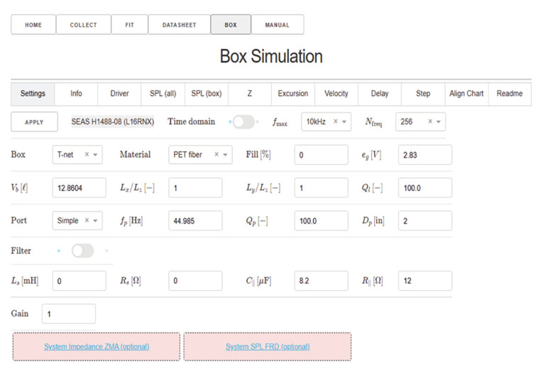
LR4Q and related alignments will soon be made available in Speakerbench [5]. Figure 1 shows a screenshot from the Box Simulation/designer. These Quasi-alignment families are “explicit” alignments in the sense that we know the polynomial coefficients. You may compare this with the Compliance Alteration technique, which describes an “implicit” alignment because you are not aiming for any particular polynomial coefficients, at least not with the provided (arbitrarily chosen) driver Qt value at hand and chosen target function. This way we may consider the Quasi-alignment families a mathematically more rigorous (i.e., well-defined) approach to explicitly target something that resembles, for example, the LR4 (Linkwitz-Riley) filter function. VC
 
References
[1] A.N. Thiele, “Loudspeakers in Vented Boxes: Part 1 - 2,” Proc. IREE (Australia), Volume 22 (1961). Republished in the Journal of the Audio Engineering Society (JAES), Volume 19, May and June 1971. www.aes.org/e-lib/browse.cfm?elib=2173 and https://www.aes.org/e-lib/browse.cfm?elib=2163
[2] R. Small, “Vented-Box Loudspeaker Systems Part IV: Appendices,” Journal of the Audio Engineering Society (JAES), Volume 21, Issue 8, pp. 635-639; October 1973.
https://www.aes.org/e-lib/browse.cfm?elib=1941
[3] R. H. Small, “Vented-Box Loudspeaker Systems Part I: Small-Signal Analysis,” Journal of the Audio Engineering Society (JAES), Volume 21, Issue 5, pp. 363-372; June 1973.
https://www.aes.org/e-lib/browse.cfm?elib=1967
[4] J.E. Benson, “Theory and Design of Loudspeaker Enclosures,” Synergetic Audio Concepts (with permission from Dr. J.E. Benson and Amalgamated Wireless Australasia Technical Review) 1993, p. 188. Speaker Builder, January 1993.
[5] Speakerbench, https://speakerbench.com
 

---

Appendix

This Scilab script shows how to calculate the quasi-alignments recursively.
About the Authors
Claus Futtrup received his MSc in ME from Aalborg University in 1997, specialized in materials science, and has worked in the loudspeaker industry since. First at Dynaudio (8 years), then at Tymphany, and subsequently Scan-Speak (8 years total), and at SEAS Fabrikker in Norway (8 years). Since 2021, he has been working at DALI as Engineering Manager of the acoustics team.

Jeff Candy received his Ph.D. in Physics from the University of California, San Diego in 1994, and is currently Director of the Theory and Computational Science Division at General Atomics in San Diego, CA. His primary work is in plasma kinetic theory and turbulence. In the audio field, his interest is the application of methods of theoretical acoustics to practical situations. Dr. Candy is a member of the Audio Engineering Society and a fellow of the American Physical Society (APS). In 2003, he received the Rosenbluth Award for fusion theory and was 2008 Jubileum Professor at Chalmers University.

This article was originally published in Voice Coil, January 2025