Simulation Techniques: Acoustical Shape Optimization for Vibroacoustics Applications

This article explores free-form and alternative optimization techniques where the topology of the geometry is given from the outset. Using practical examples, this article addresses shape optimization techniques, identifying useful types of boundaries and challenges to look out for audio product designs.
 
In a previous article, it was demonstrated how formal optimization can be used for product design of audio products such as speakerphones and waveguides [1]. The optimization approach was the so-called topology optimization technique, which is the most free-form technique in that new domains can emerge during the process and highly complex structures can arise to help meet the desired optimization targets. However, alternative optimization techniques are available such as Shape Optimization. Here, the topology of the geometry is given from the outset, such that no new surfaces will appear or disappear, but those present in the initial setup can be set free to deform as the optimization routine progresses. Typically, only a subset of the boundaries is assigned for the shape optimization with the rest of the boundaries being fixed in position.

The deformation of the boundaries can be driven by different means. In some instances, the deformation perturbation is described via polynomials, for example a Bernstein polynomial, whereas in other cases a more “free-form” approach can be chosen, see for example the COMSOL Learning Center video on shape optimization [2]. Only 2D-axisymmetric cases are considered here, but shape optimization can be used in 3D cases also, where the boundaries in question are surfaces instead of edges.

As with topology optimization, the procedure entails certain objectives and constraints. The so-called objective function is a mathematical description of one or more targets that are sought, for example a particular on-axis pressure, radiation patterns, and similar. The constraints can be related to the geometry to make sure that within the optimization routine no boundaries will leave a certain “bounding box” or that boundaries will not overlap each other. In general, the more targets and constraints the optimization setup has, the more difficult it will be to find a solution, so it will often be somewhat of an iterative process to set up an optimization routine, especially for industry cases.

The focus for the cases is not a particular objective function as it will typically take a lot of time to reach some desired goals, which is simply not feasible to spend here. Instead, the principles are illustrated, such as which types of boundaries can be used in a shape optimization setup and which problems to look out for when doing shape optimization.

Tweeter Waveguide
A first example is given here with a tweeter sitting in a waveguide. It should be noted that my definition of a waveguide is quite loose in that it is simply any geometry modifying the acoustic field in front of a transducer, whereas others working in the field of waveguides and horns would have much more stringency in their definitions, see for example articles written by Bjørn Kolbrek [3], [4] and Earl Geddes [5] for the theoretical aspects of waveguides and a discussion about assumptions and limitations. My view here is different in that much of the work that I do on loudspeakers are for applications that are not related to traditional in-home audio, such as highly constrained geometries for gaming equipment, headphones, and even rodent-repellent devices to name a few, and so I have become less sensitive to how a geometry is categorized formally. In general, the theory on the topic of waveguides starts out with a geometry that aligns with a particular coordinate system, as seen in Kolbrek’s article [4].

However, there is an assumption that the sound field in question also follows said coordinate system, without necessarily considering that: 1) the sound field is generated by a physical transducer of some complex shape, and so the sound field is unlikely to adhere to a particular coordinate system near the transducer; and 2) the waveguide has to end somewhere and open up into a free space of sorts, so there is a transition in which the sound field has to take on another character. The analytical expressions are therefore not generally enough to find an optimal geometry.

Also, while one might be able to find a well-behaved waveguide via such methods for a single tweeter setup in a loudspeaker, there will be other situations such as for in-car audio where the environment, starting geometry, and number of drivers differ immensely from this more prototypical setup, and so there will not be any analytical expression available from which to start. Here, a formal optimization routine with an algorithm deciding each new deformation of the waveguide based on the former deformation’s effect on the targets can be utilized instead.

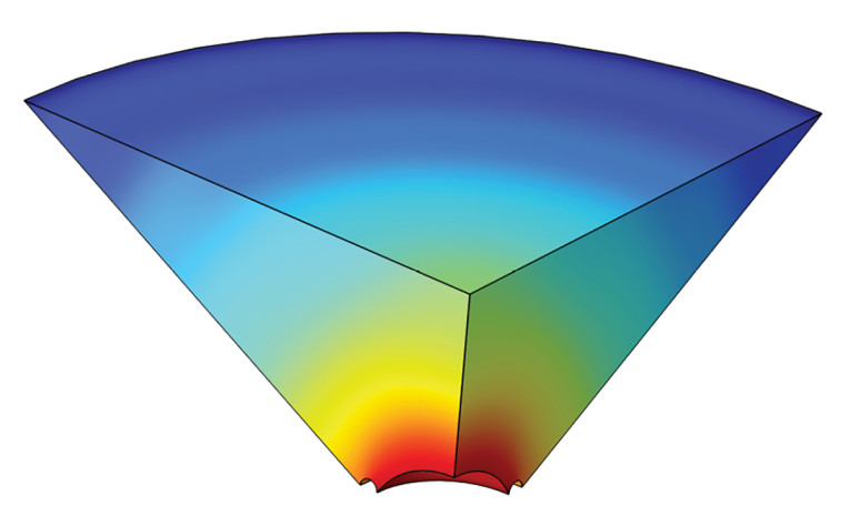
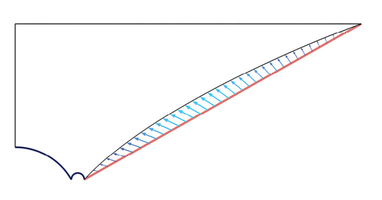
The setup in question is shown in Figure 1, where a tweeter is recessed in a waveguide with straight-line boundaries in its initial state opening to a baffled 2π domain. The red boundaries indicate where the shape optimization is allowed to take place, and it should be noted that the underlying simulation is 2D-axisymmetric only, with the 3D views being revolved views. The tweeter is not included explicitly as geometry, but its interfacing boundaries can be seen, and they are given a simple acceleration boundary condition to drive the sound. For a particular tweeter one can include its Thiele-Small parameters in the boundary condition to include the two-way coupling taking place at these boundaries, or alternatively include the tweeter geometry and physics.
 
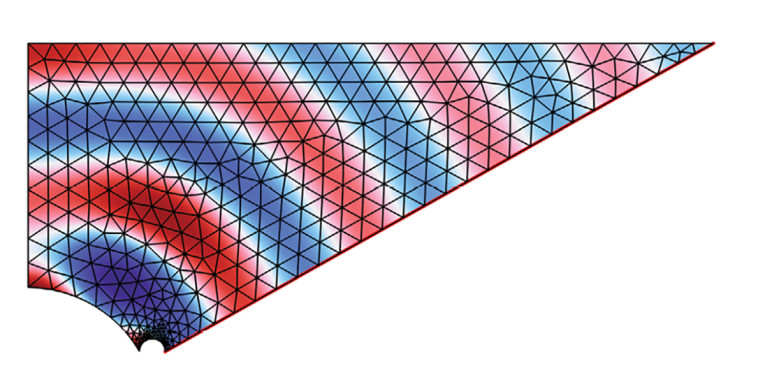
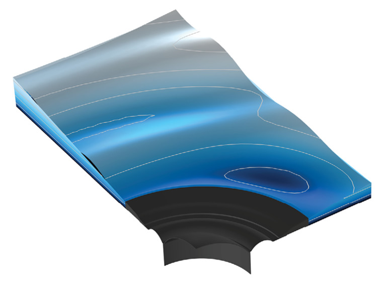
One complication of shape optimization via the so-called Finite Element Method (FEM) is that there is an underlying mesh as shown in Figure 2. This mesh will deform during the shape optimization procedure, and there is a risk that some of the elements in the mesh will be so heavily deformed that the FEM equations cannot be solved, and the solver comes to a halt. So meshing is one point that must be considered in setting up a robust optimization run, especially for complex 3D cases.
 
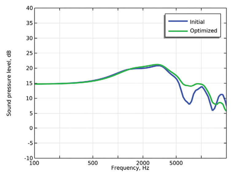
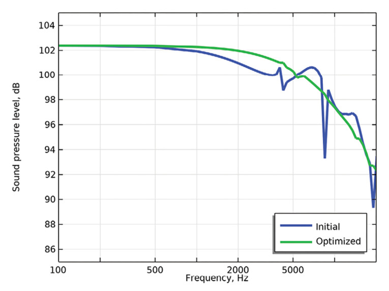
The objective function for this case could involve a multitude of targets regarding on-axis and off-responses, but here only the on-axis response was sought improved, as seen in Figure 3. The targets will vary from client to client and case to case; sometimes they can be reached to an extreme degree, and sometimes it is more of an ill-posed problem that is sought solved, possibly without a satisfactory solution in end. Again, the focus here is on the setup and how shape optimization can be applied, and not so much on the actual design work and the final results.
  The optimized 2D-axisymmetrical geometry is overlaid with the initial geometry in Figure 4 with the tweeter boundaries in blue and the initial boundary being optimized in red. It shows how the initially straight-line boundary is deformed into a different shape to modify the sound field.
  While the case is fundamentally 2D-axisymmetrical, it is also possible to do shape optimization for 3D cases, where the boundaries in question are surfaces, as illustrated in Figure 5.
  Compression Driver Phase Plug
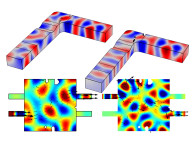
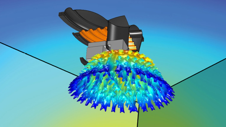
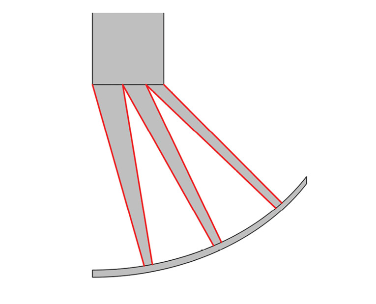
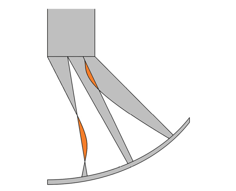
Another example is shown here for a so-called compression driver. This type of driver has a rather large membrane/diaphragm compared to the outlet of the phase plug it sits in, hence the “compression” part. The phase plug is here sought shape optimized to meet a certain target, and the starting geometry is based on Samsung Research America’s work [6].

The phase plug has three channels in this case as illustrated in Figure 6. The red boundaries are to be deformed via the shape optimization.
  This case presents some new challenges compared to the previous one. Now, the boundaries are at risk of overlapping, and in two different ways. One issue is that boundaries within one phase plug channel can overlap and block off the channel. In that case the simulation may stop as the simulation setup will no longer be valid. Another issue is that two plug passages can overlap, in which case the solution process may end successfully, but with a final geometry that is not physically realizable. The two situations are illustrated in Figure 7. To handle such overlaps different tactics can be employed, such as constraining the minimum distance between boundaries and/or pairing up deformations.
  With the overlap issues handled, we can find a solution for the phase plug such as shown in Figure 8, where the straight lines have deformed into new smoothly curved ones.
  The associated sound pressure level (SPL) is shown in Figure 9, where the optimization has clearly led to a much smoother response. The plane wave tube terminating the phase plug could of course be replaced by a situation where the phase plug sits in a horn with free radiation conditions, but the shape optimization setup would be the same.
  Cone Geometry
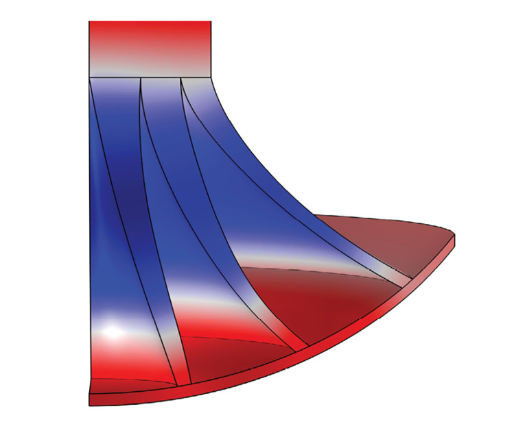
For the previous examples the boundaries used for the shape optimization were “acoustical” in the sense that on one side of them there was an acoustical domain, and on the other there was no defined physics. However, that does not always have to be the case. Instead, the boundary may be a structural mechanics boundary that couples to an acoustics domain, for example for a cone geometry as shown in Figure 10.
  We immediately see that we can run into some trouble for such a case. For one, the cone is heavily deformed and may be difficult to manufacture. Also, the cone and the surround couple in a delicate way, which will now be disturbed by a shape optimization setup done too “academically” without considering the engineering aspects. Finally, for an acoustic-structural boundary there may be numerical issues regarding optimization and calculating sensitivities, and so it may be a better choice to perform the shape optimization on the structural mechanics only and couple to an implicit acoustics domain via a Rayleigh integral [7]. Those details will not be discussed here. So, while it is possible to deform such an acoustic-structure interface boundary, one must take care in the execution.

Acoustic Lens for Tweeter
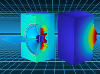
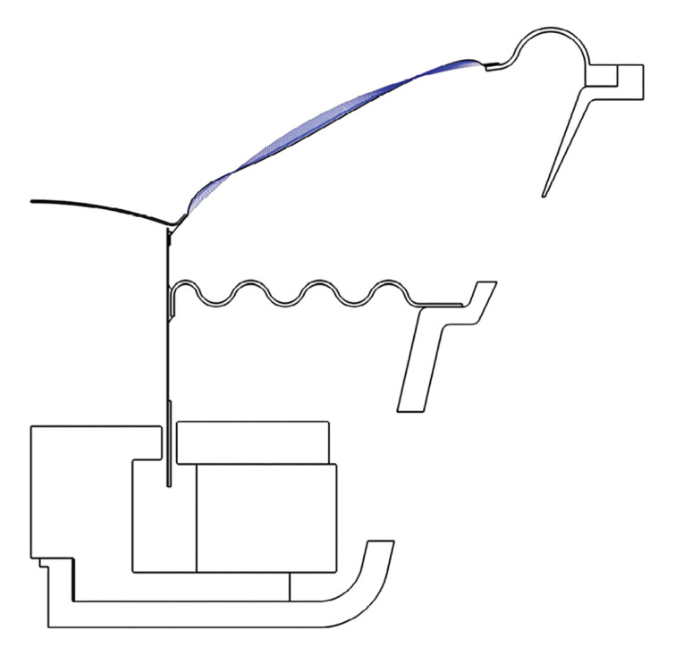
For a final example, an acoustic phase plug/acoustic lens for a tweeter is designed. Here, the boundaries are acoustical, but they have been added manually to the existing geometry to achieve some new functionality. This will typically be based on some a prior knowledge, for example from a previous topology optimization hinting toward a specific design or perhaps from a trial-and-error approach. The resulting geometry is shown in Figure 11, where the red boundaries indicate a hard-walled geometry to be put in front of a tweeter to manipulate the resulting sound pressure levels.
 
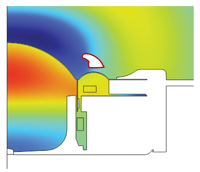
The starting point for the boundaries was found via a preceding topology optimization setup with the same target, which is a major assistance to the shape optimization. If one simply starts out with circular geometries in the same general location with its boundaries free to deform via shape optimization, the resulting optimized geometry might be quite “ellipse-like” and not so complex as the shown geometry, especially if using polynomials for the deformation, as they cannot wrap around themselves, since for any proper function there can only be one output value to any one input value. So, while the principle of shape optimization has been illustrated here, there are many more intricacies to consider.

Conclusion
It has been demonstrated how the shape optimization technique can be used for product design in the audio industry. Just as with topology optimization, new designs can be found that would often be very difficult to arrive at using traditional engineering approaches.

As with any optimization technique, or indeed any new method, it is important to not forgo traditional engineering methods and analytical expressions when seeking a solution. Sometimes a new “hammer” will make all problems seem like nails, but optimization will often leave you one or more steps removed from the analysis of why a certain geometry worked in the first place. This is a balancing act: If the solution space is vast, optimization can give you answers that trial-and-error would never have provided, although the final geometry may be so complex that it is not possible to describe in detail how it works. On the other hand, more standard engineering methods can often be the better way to go, especially when similar problems have been encountered and solved in the past.

Finally, it should be noted that there is a potential for combining shape optimization and topology optimization, which would make for even more intricate geometries. Also, some versions of shape optimization are specialized in way such that some closed boundaries can be removed if they are small enough to not affect the sound anyway, see for example the work of Peter Risby Andersen [8].  aX

References
[1] R. Christensen, “Acoustic Topology Optimization for Vibroacoustics Applications,” audioXpress, April 2023.
[2] K. E. Jensen, “Introduction to Shape Optimization,” COMSOL.
[3] B. Kolbrek, “Horn Theory: An Introduction, Part 1,” audioXpress, March 2008.
[4] B. Kolbrek, “Horn Theory: An Introduction, Part 2,” audioXpress, April 2008.
[5] E. Geddes, “How Horns Work Revisited,” audioXpress, December 2008.
[6] A. Bezzola, “Numerical Optimization Strategies for Acoustic Elements in Loudspeaker Design,” Audio Engineering Society 145th Convention, New York, 2018.
[7] R. Christensen, “Loudspeaker Driver Displacement Decomposition,” audioXpress, January 2023.
[8] P. Risby Andersen et al., “Experimental characterization of a shape optimized acoustic lens: Application to compact speakerphone design,” The Journal of the Acoustical Society of America, Volume 154, No. 4, pp. 2351-2361, 2023.

This article was originally published in audioXpress, February 2024