Any remedies to lessen this computational load can improve the overall workflow, and design changes can be evaluated faster, so it is always a good idea to seek ways to simplify model complexities. Here, we will have a look at how to reduce computational costs utilizing symmetry schemes and dimensional reductions techniques, and potential issues associated with them.
All aspects of any transducer or any other product are essentially three-dimensional, and so to get the full picture of its operation, any simulation should essentially be carried out utilizing the full geometry. However, in some instances symmetry conditions can be invoked to reduce the total number of degrees-of-freedom in the computational setup. There are several considerations regarding whether the symmetry in geometry, boundary conditions, load/sources, and/or field, or only in a subset of these.
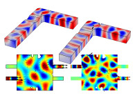
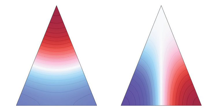
An example of this is shown in Figure 1, where a geometry has a symmetry plane, but applying a symmetry or “mirror” condition on the midline and solving this as an eigenmode problem using only half the geometry in the simulation would not return all possible modes, as some will have anti-symmetry in the field. So, for each symmetry seen in a geometry, one must carefully consider if several runs with different types of symmetry conditions are needed to reach the same total result as the full geometry would. This becomes especially important for some sub-physics such as structural mechanics or microacoustics, where shear forces come into play.
For structural mechanics there will typically be one degree-of-freedom per dimension, such that for a three-dimensional problem, one needs to resolve three displacements per point in the geometry, so any computational costs saved here will benefit the user. For standard pressure acoustics, there is only one degree-of-freedom to consider, namely pressure, but while there may be less saved in general by invoking symmetries, the acoustics domain are often rather large and could be the bottleneck in the setup. In general, one must consider which types of physics are involved, and which type of study is being run, before naively applying symmetrical conditions based on geometry only.
Different Conditions
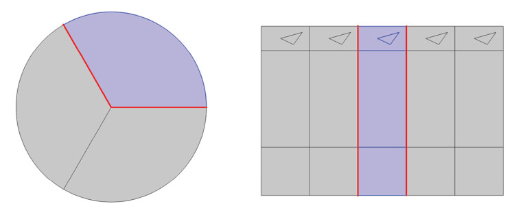
Different conditions can sometimes be utilized in similar situations where a repeating pattern is present in the geometry, the so-called periodic conditions. These can be simple mirror conditions, anti-symmetry, or more involved such a Floquet conditions for repeating patterns on a grid. These periodic conditions may be applicable to such structures as those shown in Figure 2, but again this must be evaluated based on the physics, type of study, boundary conditions, and loads in question. Also note that if optimization is added on top of the simulation, additional considerations must be made, as the optimization may have additional symmetries [1].
Utilizing symmetry planes can reduce the overall computational cost by only considering a subset of an original geometry, but the dimensions of the remaining subset will be the same as the original. A different approach to reducing complexity in a simulation is what can be called “dimensional reduction,” where a three-dimensional domain is modeled using lower dimensions for some or all physics domains involved. This is commonly used in structural mechanics where “plane strain” or “plane stress” assumptions are made to reduce three-dimensional problems to two-dimensional ones, or in acoustics where for example a three-dimensional duct problem may be reduced to a one-dimensional one, under certain conditions. For transducers, where more than one physics is typically involved, several different dimensional reduction combinations can be constructed, and this will be illustrated here with a traditional moving coil loudspeaker problem used as the prototypical example.
One Common Dimensional Reduction Approach
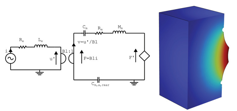
One common dimensional reduction approach is to assume zero-dimensional behavior for electromagnetism and structural mechanics, with the effect of the acoustics environment included to some degree in a zero-dimensional fashion locally. This is done via lumped components, see for example [2], where the electromagnetic effects are included via one or more resistors and ditto inductors, and a total moving mass, a total stiffness, and a total loss are found for the loudspeaker driver, typically via measurements. The stiffness comes mainly from the spider and the surround, while the mass comes from all moving parts. While these parts each have their own mechanical characteristics, here they are lumped into single components, such that no modal behavior other than the fundamental for a single degree-of-freedom spring-mass system is included in the model.
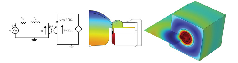
This is illustrated in Figure 3. The moving coil transductance principle is non-reciprocal and a coupling between the electromagnetics and structural mechanics is needed where the effort variable on the electromagnetic side voltage is coupled to the flow variable velocity on the structural mechanical side, and the flow variable current is coupled to the effort variable force, respectively. A so-called gyrator is utilized in the lumped circuit to obtain this coupling. Here, the zero-dimensional domain electromagnetics is coupled to the zero-dimensional domain via linking the mechanical velocity and the voltage u’ in the circuit as:
Blv = u’
Additionally, the force applied to the vibroacoustics is linked to the current as:
F = Bli
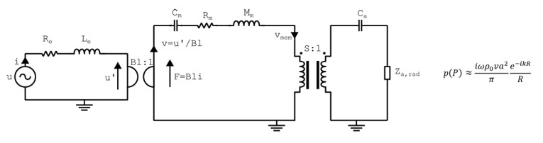
The coupling between the mechanical and the acoustical domains is then implicitly included in that the impedance loading (typically denoted as “mass loading”) from the acoustical environment on to the structural mechanics domain is included via lumped components, such as capacitor for the compliance from a rear enclosure, and simple radiation conditions included via an impedance. Analogously, the mechanical velocity found in the lumped circuit is assumed to be common for all parts, including the cone, and so this velocity is related to the acoustic excitation. However, the pressure of interest will almost always be at a certain distance away from the transducer and this pressure cannot be found locally in the lumped circuit.
This issue is typically dealt with via assuming the transducer acting as simple monopole source or a piston placed in a baffle and having an analytical expression for calculating the pressure at a distance. In the latter case, the Rayleigh integral is employed and simplified:

More Complicated Acoustic Environments
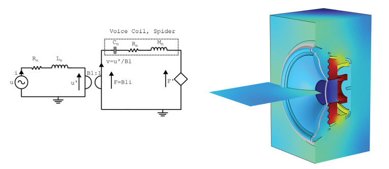
For more complicated acoustic environments, to include diffraction for the enclosure and perhaps the inclusion of a complex rear chamber geometry, a different dimensional mapping can be utilized, where zero-dimensional components for the magnet system and structural mechanics part are used. These are then coupled to a three-dimensional acoustical domain, possibly with its own symmetry planes. The coupling takes place across the cone surface, and there are no moving parts in the finite elements analysis, although it may be advantageous to keep all explicit geometry parts to have the acoustics at the rear of the transducer better represented. This setup is shown in Figure 4, where the three-dimensional acoustic field is resolved with a coupling to the lumped mechanical components.

The lumped velocity is driving the acoustical velocity across the cone, surround, and dust cap, and here one needs to make choices about how this velocity is distributed and if the scalar velocity in the lumped model relates to a normal or an axial direction.
The coupling can be two-way in that not only does the zero-dimensional velocity drive the acoustical energy input, but also the pressure conditions across the cone can be coupled back to load the electro-mechanical system, so that:
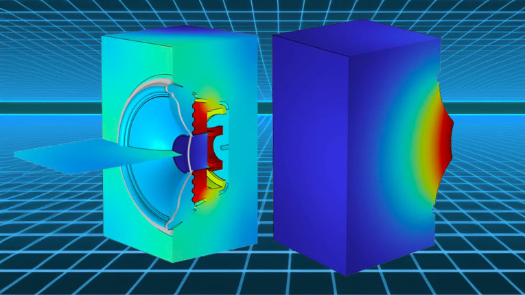
The couplings for the moving coil transducers shown in Figure 5 are sequential in that there is an interface between the electromagnetics and the structural mechanics, and between the structural mechanics and the acoustics. The dimensional splitting can be done directly at those interfaces, but there are alternatives such as splitting the dimension in between the acoustical parts, as just shown, but also in between mechanical parts. This was described in the literature [3] as a “hybrid” model around the time some of us were also doing it in the industry, and was years later described again [4], although the method was the same.
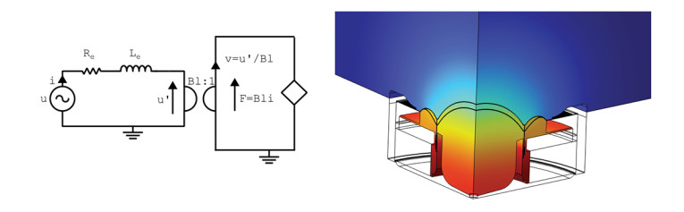
The idea is to include the vibrating surface, typically cone, dust cap, and surround, as explicit domains, and lumping together the remaining moving parts on the rear, such as the spider and the voice coil (former plus windings), alongside a lumped magnet system. This setup is illustrated in Figure 6, where the cone, surround, and dust cap are now moving parts with structural mechanics physics applied, while the remaining mechanical parts are found in the lumped circuit. While not emphasized in the literature, it has already been mentioned here that it may be important to have the lumped parts still included as geometry, as to better capture the rear acoustics, where the parts may form somewhat closed off regions with distinct resulting pressure characteristics. Also, as the former, windings, and spider have their own distinct mechanical modal behavior, these can influence the overall displacement from a structural mechanics perspective, and hence affect the sound pressure, and these effects are excluded in this model.
If all mechanical components are included explicitly, a setup is had, as illustrated in Figure 7, where only the electromagnetics are lumped, and the structural mechanics and acoustics are included in either 2D-axisymmetrically or three-dimensionally.

Alternative Mapping
This leads to an alternative mapping that I have not seen described in the literature, shown in Figure 8. Here, the magnet system is included as lumped components, although it could be included in the 2D-axisymmetrical model for more elaborate magnet setups. The 2D-axisymmetrical domain includes all moving parts explicitly, and so modal behavior is included, albeit excluding circumferential variation. These variations may not be important as these modes are not necessarily excited much, and/or do not contribute much to the sound field, although this must be evaluated on a case-by-case basis. The rear acoustics geometry may be highly intricate, and can for example include microacoustics effects, porous materials, ferrofluids, or other characteristics that are not easily lumped.
Finally, the front acoustics geometry can be arbitrarily detailed, for example including enclosure diffraction, phase plugs, or living room or automotive environments. The transducer can thus be included in a very elaborate manner, while still saving substantial computational cost by only resolving it in 2D-axisymmetry, or 2D, depending on the transducer type, while the acoustic effects are captured near-perfectly. Different variations of this can be made, for example if the rear acoustics is simple enough to go into the lumped model, or alternatively too complex to be axisymmetric, such that the same approach as for the front acoustics is applied to the rear utilizing three dimensions for all acoustics domains.
This type of dimensional mapping is not trivial to set up, as the meridional velocity distribution on the transducer surface must be mapped to the corresponding meridional and circumferential points in the acoustics domain. It may be necessary to also have a two-way coupling incorporated. However, this overall strategy can take a simulation from requiring a high-performance cluster to solve, to solving locally on a more modest computer, and it is especially useful if additional studies such as topology optimization [5] are applied on top of it.
Conclusions
For all dimensional mapping strategies shown here, one must take care of the scalar and vector aspects of each sub-physics. Voltages and currents in a lumped model are complex scalars in zero dimension but they have signs relative to some arrow indications in the schematics. For any lumped model representing mechanical or acoustical parts, these signs relate to a particular direction, such as normal or axial, for underlying complex displacement vectors, or positive/negative aspects of scalar pressure fields.
Assuming standard acoustics, only normal displacements create sound, but if microacoustics effects are to be included, both normal and tangential displacements must be included. Also, single forces in a lumped circuit may be calculated from integral values coming from pressures in a three-dimensional domain. Getting all these signs and directions correctly implemented is crucial for the dimensional mapping to work.
For other transductance principles than the moving coil used as an example here, such as electrostatics or piezoelectric, the dimensional mapping will be different, and one needs to consider, for example, that they may or may not be reciprocal in nature. I am planning an article series on transductance principles, to go into more of these details. aX
References
[1] R. Christensen, “Advancements in Acoustical Topology Optimization,” COMSOL Conference 2023, Munich, 2023.
[2] R. Christensen, “Lumped Element Modeling of Transducers,” audioXpress, March 2023.
[3] M. Pasi and M. J. Herring, “A Hybrid Electroacoustic Lumped and Finite Element Model for Modeling Loudspeaker Drivers,” Audio Engineering Society 51st International Conference, Helsinki, Finland, 2013.
[4] D. G. Nielsen, P. R. Andersen, J. S. Jensen and F. T. Agerkvist, “Estimation of Optimal Values for Lumped Elements in a Finite Element - Lumped,” Journal of Computational Acoustics, Volume 28, No. 2, 2020.
[5] R. Christensen, “Acoustic Topology Optimization for Vibroacoustics Applications,” audioXpress, April 2023.
This article was originally published in audioXpress, June 2024