Engineering is to a large degree the combined output of education and experience. If you are designing transducers, you need academic knowledge about acoustics, electronics, transductance principles, modeling and so on, but you also partly rely on the experience you have accumulated of a more experimental and empirical kind and you use solution strategies from previous projects to solve the problems at hand.
Oftentimes, however, the combination of academic and experimental knowledge is not enough to clear a direct path toward a product or to solve a problem in a straightforward manner. That can be the case when there are many degrees of freedom, i.e., parameters that can be changed in a system and when several targets are sought at once. In such cases, changing one parameter at a time will not be feasible for finding an optimal solution, as the optimum value of one parameter will depend on several or all of the other parameters. A trial-and-error approach could then be used, but that can cause new issues, as you can easily end up spending a lot of time without getting any closer to a solution. More systematic approaches such as Design of Experiments (DOE) [1] may be helpful if the number of parameters is limited, but many design problems have so many design variables that a simple combinatorics analysis will show that it could literally take years to explore the full solution spaces, even when using simulations instead of experiments.
In cases with a large solution space and several complex targets, it is advantageous to turn to “formal optimization.” By formal, I mean a procedure driven by mathematics with one or more objectives (targets), and one or more constraints, typically defined within some finite element modeling framework. With the optimization problem formulated via mathematics, a computer algorithm can be utilized to solve the problem.
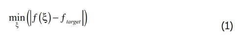
For any type of optimizations, one must have an objective function defined via a mathematical expression that describes the desired targets. This can be quite difficult to achieve. It could be that you are interested in having a flat on-axis sound pressure, and a particular directivity index, alongside one or two more targets, and some of these may be easy enough to formulate in a sentence but not as mathematics. Once defined as an expression, the objective function can be minimized or maximized, such as the difference between some target value ftarget and a variable of interest f(ξ) being a function of the design variable ξ to be explained shortly. A minimization of an objective function could in principle look like Equation 1:
With a proper target function defined, there typically are also certain constraints to consider. That could be how much of the domain assigned for optimization can take on a “solid” form as shown shortly, or other constraints involving the acoustic variables. With the targets and constraints defined mathematically, and the general finite element setup in place, the optimization can be run and while there is no guarantee for finding an “absolute” or global minimum, the optimization routine should at least find a local optimum.
For so-called topology optimization problems, a design variable ξ is defined via a field that varies in an assigned optimization domain [2]. It can take on values between zero and one, and while it is a continuous field, the optimization routine is set up to prioritize values being either close to zero or close to 1. This will ensure a more binary field where a 0 will be interpreted as being air and a 1 is interpreted as a rigid solid mechanics structure, although in the simulation it is a fluid; a fluid with very high density and ditto bulk modulus; the “stiffness” of the fluid.
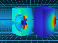
For a design variable field that is close to binary across the domain, a solid mechanics structure of the same shape as the field can be expected to result in similar optimized results, but since it is generally not possible to have a completely binary field, the resulting geometry should always be tested by exporting the field and then import it interpreted as a solid structure in a subsequent simulation. In Figure 1, an example of such a two-dimensional design variable field is shown with black parts being interpreted as solid parts. The sound field can also be seen, revealing the objective function used in the simulation; to convert a non-planar sound field from the left to a planar one on the right. This already alludes to what can be achieved with optimization and how this very non-trivial problem can be solved with the proper optimization setup.
Topology Optimization Examples
Several acoustic topology optimization examples are shown now, where the simulation software COMSOL Multiphysics was used.
Tweeter Phase Plug
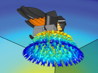
The first example is taken from a COMSOL Conference paper [3]. A tweeter geometry was made with realistic parameters and materials, and its resulting sound pressure level (SPL) is sought to be modified via acoustic topology optimization. A domain in front of the tweeter was assigned as the optimization domain, and an objective related to the on-axis SPL was defined mathematically. The resulting “phase plug” geometry is shown in black in Figure 2, where the optimization routine has found that this new geometry placed close to the tweeter “surround” will modify the SPL to best meet the set objective.
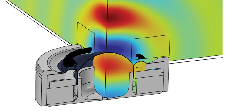
The optimization field for the design variable was exported as a geometry, and a new simulation was run to test the topology optimized geometry. The on-axis SPL before and after adding the phase plug are shown in Figure 3 and the overall level is flatter and higher after the optimization.
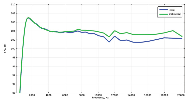
It should be noted that while your objective(s) may be met to some acceptable degree, one should always investigate if other quantities have changed for the worse because of the optimization. In this case it would be informative to look at radiation patterns and off-axis responses before and after optimization to check that any changes are acceptable. If something has changed negatively, it may be necessary to reformulate the objectives and/or constraints to include the new information and run the optimization again. Also, the fact that the geometry is placed this close to the tweeter could point toward an issue with the displacement phase on the tweeter surface [4], and so it might be that the tweeter itself can be modified in such a way that the phase plug is no longer needed. In such cases the optimization will still have aided in the design work, and so it is not always the aim to use the topology optimized geometry directly, but instead as inspiration for simpler changes.
Speakerphone
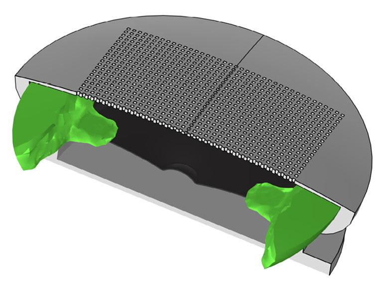
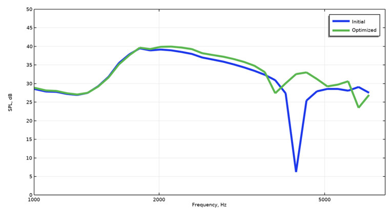
A generic speakerphone was made in which the front domain was assumed available as a topology optimization domain. The initial response on-axis is shown to have a dip at around 4kHz, and the objective here is to have a flatter response on-axis without this dip. With the speakerphone sitting on a table, on-axis pressure may be less important than off-axis responses, but it is chosen here anyway to illustrate the principles of the optimization.
The speakerphone is shown in Figure 4 with the geometry resulting from the acoustic topology optimization in green. The SPL is flatter after the optimization as shown in Figure 5 with the dip removed from the response. Instead of exporting the geometry parts from the optimization and using them directly in a design, their shape and placement could again be used as inspiration for where to place components that anyway must be in the speakerphone, such as the electronics. And for this case it could also be that traditional engineering methods would have revealed the underlying modal acoustical behavior and a similar solution could perhaps fall out of this analysis. As already mentioned, for certain problems the combinatorics involved will make it impossible to find the proper distribution of material by a trial-and-error approach, and one such example is now presented.
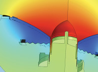
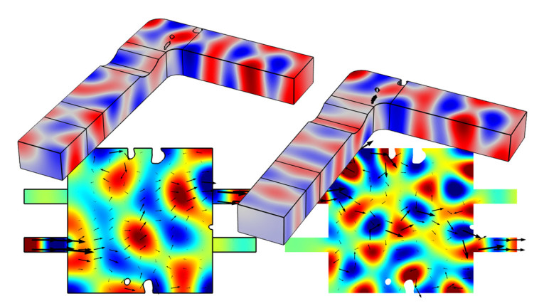
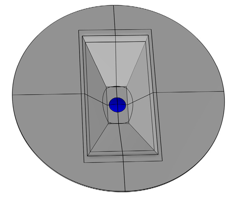
A tweeter is located at the bottom of a waveguide, and it is assumed that the waveguide cannot have its shape changed. Instead, the air domain in the waveguide is assigned for topology optimization, and so a phase plug can grow out of this domain to obtain certain targets regarding SPLs and directivity. While for a traditional loudspeaker this type of design would probably not be done using topology optimization, one can imagine situations such as loudspeakers sitting deep in a TV or other products with a complex geometry, where there is no other option than to change the topology in an acoustical path. Also, different phase plugs could be found that meet different objectives and delivered alongside the product as a way for the user to change for example the directivity of the loudspeaker.
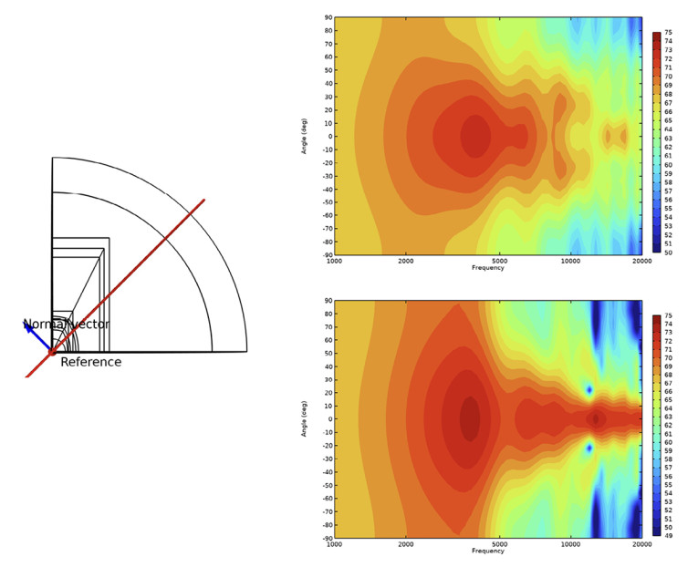
The initial setup is shown in Figure 6 with the tweeter indicated in blue sitting in a rectangular waveguide. There are several objectives involved here regarding SPLs and the directivity index, with the air inside the waveguide assigned available for topology optimization. The resulting phase plug has a very distinct geometry as shown in Figure 7, which could not have been found using traditional engineering methods, and it is unique to this setup. The directivity is shown in Figure 8, where a clear improvement in the radiation at higher frequencies is seen.
Changing the objectives even slightly will result in a different phase plug topology, and in that sense a geometry found via optimization may not lend itself well to “reverse engineering,” where the functionality can be deduced after the optimization. That may be discouraging in that it is always best to understand the underlying principle of any added geometry, but this must be weighed against not finding a solution at all. Also, there will certainly be instances where the optimized result will be easier to deconstruct, and simplified versions that are more easily manufactured may then be made. But in the current case with a complex initial geometry and multiple objectives, one simply must accept the geometry output as it is.
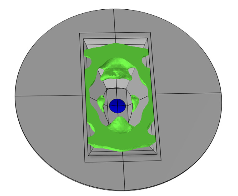
For wave propagation problems such as the acoustics involved in the present cases, every small detail of the resulting topology is important, and so the geometry needs to be very distinctly represented or else the manufactured part will not meet the targets when installed. Also, you might end up with parts of the optimized geometry floating in space without attaching to any other parts. In such cases, it will be necessary to modify the geometry so that these parts are connected. For the present case, all the phase plug parts touch the waveguide and so the waveguide could be made to have this shape, but there is no guarantee for this connectivity in the typical topology optimization setup.
Conclusion
Acoustic topology optimization represents a new tool in the tool box for vibroacoustics engineers. It does require a lot of knowledge about the topology optimization procedure as many aspects are involved such as filtering needed to obtain a near-binary design variable field. The general acoustics involved should be well understood alongside the traditional engineering methods to determine if a case is suited for formal optimization or not. While still not commonplace, I expect that in the coming years we will see more cases where acoustic topology optimization is used in product development for loudspeakers and vibroacoustics applications in general. aX
References
[1] J. Antony, Design of Experiments for Engineers and Scientists, Elsevier Science & Technology, 2014.
[2] M. Bendsøe and O. Sigmund, Topology Optimization: Theory, Methods and Applications, Springer, 2002.
[3] R. Christensen, “Acoustic Topology Optimization - Implementation and Examples,” in COMSOL Conference, Cambridge, MA, 2019.
[4] R. Christensen, “Loudspeaker Driver Displacement Decomposition,” audioXpress, January 2023.
This article was originally published in audioXpress, April 2023