A balanced armature (BA) transducer, also called a balanced armature speaker (BAS), is a miniature loudspeaker commonly found in earbuds, hearing aids, and in-ear monitors (IEMs) due to its compact size and high performance [1]. It belongs to a group called moving-iron speakers, which is the earliest type of electric loudspeaker to have been invented. With a history that can be traced back to its application in the early telephones invented by Alexander Graham Bell, moving-iron drivers are electromagnetic (EM) transducers that rely on the magnetic forces (the Maxwell stresses) between magnetized bodies for motion.
Nowadays, BA transducers have evolved to become known for their small size, light weight, low distortion, and high electrical efficiency. A schematic representation of a modern transducer can be seen in Figure 1. It contains an armature (made of a magnetic alloy) that runs through a coil and is balanced between two permanent magnets. When an AC voltage is applied to the coil inducing an AC current, the arm is magnetized and alternating magnetic fluxes are generated. This makes up a magnetic circuit with a strong interaction between the AC magnetic field (generated by the coil) and the DC field of the permanent magnet. This in turn generates an alternating push–pull force on the armature. Since there is a driving rod/pin connecting the arm and diaphragm, the movement of the arm is passed onto the diaphragm, resulting in sound waves.
There is a growing trend to adopt multiple receivers in the same device, with each covering a specific target frequency band and working in combination to deliver the best overall sound. The pursuit of higher sound quality and smaller geometry size in each design requires a good understanding of the working mechanisms as well as many tests and trials, which is no different than the requirements of Bell’s time.
However, with the development of modern technologies, engineers can now use numerical simulation to gain a better understanding of the physical phenomena involved, try out different ideas, and prototype with ease in a virtual environment. In the virtual world, one can freely change the structure, material, and operating conditions of a device or, if available, even use an optimization algorithm included in the simulation software to find an optimal design. In general, numerical simulations can be introduced at every stage of the design cycle, which often results in fewer physical prototypes; lower costs; faster time to market; and most importantly, better products. It can be extremely useful in the design of devices that involve multiple physical phenomena affecting one another, such as in balanced armature transducers.
When using simulations to evaluate a BA transducer’s performance in a specific application, a lumped circuit representation of the transducer is often adopted to study its interaction with other components in the system [2,3,4]. This lumped approach provides a quick and convenient way to perform a system analysis. However, when it comes to the design of the transducer or optimizing certain components for a specific frequency band, a full and detailed electrovibroacoustic analysis including all the acting electromagnetic and mechanical components of the transducer becomes necessary.
This type of detailed analysis provides an understanding of how some key design parameters affect the electromagnetic properties, the vibroacoustics behavior of the moving parts, the damping mechanisms, and the acoustic response. With a specific goal in mind, such a detailed model can also be used for an optimization analysis of certain driver components to determine the ideal dimension, shape, or topology and study the nonlinear distortions resulting from large deformations.
Now let’s investigate how to set up a finite element model for such a detailed analysis [5]. The modeling example presented in this article is conducted in the frequency domain, assuming small perturbations and linearity under harmonic excitations.
Underlying Physics and Their Interplay
A full electrovibroacoustic analysis requires solving a fully coupled model that combines the electromagnetic field with structural vibrations and acoustic radiation. For the electromagnetic part of the simulation, Maxwell’s equations are used to describe the magnetic flux in the air and the solids. However, due to the dynamics of the analysis, the magnetic and electric fields are coupled. Some of the most important electromagnetic quantities encountered in the analysis are the magnetic field intensity and flux density, the current density, the electric field and displacement, the electric conductivity, and the driving frequency.
The transducer contains different material types, and their electromagnetic behaviors can be described with various electric and magnetic constitutive relations, as well as electric conduction models. For example, you can prescribe a remanent flux density for the permanent magnetic, use a nonlinear B-H curve to describe the soft iron properties for the pole piece, and use a linear relation for other materials. In the coil domain, a homogenized current density can be prescribed.
Structural Vibrations
The vibrations in the structural domains are described by the dynamic force balance determined by Newton’s second law. Some of the most important mechanical quantities are the mass density; displacement field; stiffness; strain; and body load, such as the magnetic force induced inside the arm. The behavior of different solid materials can be described with different stress–strain constitutive relations. In this case, it is sufficient to use an isotropic linear elastic material model that assumes a linear relation between the stress and strain (i.e., the stiffness tensor is constant).
A nonlinear strain-displacement relation is used, which is necessary when the linear vibration model needs to be solved in a deformed geometry. This is required in this example because the armature experiences static Maxwell stresses, and therefore static deformation, in the permanent magnetic field. The static solution should be calculated first and then used as the linearization point for a frequency-domain perturbation study. This nonlinear formulation also allows for a large static deformation when the relation needs to be described in a deformed geometry.
Acoustics
For the acoustics in the air domains, special attention is needed in the slit-like narrow regions to capture the correct thermoviscous boundary layer losses. The acoustics in these areas are best described by the full set of linearized Navier–Stokes equations in quiescent background conditions (in other words, the governing equations describing the thermoviscous acoustics) [6]. For a frequency-domain analysis, the Helmholtz equation and an equivalent fluid model that adds or smears the boundary layer losses onto the bulk of the fluid are used.
This is because analytical expressions exist for many geometries where the losses associated with the acoustic boundary layers are introduced through frequency-dependent, complex-valued speed of sound and density. These are known as low-reduced-frequency (LRF) models [7,8,9] and are less computationally expensive compared to a full, detailed thermoviscous acoustic model. Some of the most important acoustical quantities are the acoustic pressure, fluid density, speed of sound, and driving frequency. In the narrow regions where an LRF model is used, the density and speed of sound become complex-valued quantities to model the desired losses.
Interaction Between Deformable Solids and Magnetic Fields
When magnetized by an AC current applied to the coil, the armature lying in the air gap experiences the Maxwell stress that forces it to move. This stress includes two contributions: one is volumetric, accounting for the stress that is present inside the magnetized bodies, and the other is on the surfaces, accounting for the stress that comes from the interactions with the surrounding magnetic field.
In addition, the solid deformation influences the material magnetization, which can be included by taking the EM vector components on the material frame [10]. Furthermore, the varying air gap introduces a change in the magnetic flux circuit (i.e., a varying reluctance), and this effect can be captured by modeling the geometric change in the air domain. Therefore, the magnetic model should be solved in a deformed geometry to correctly simulate the effects from solid movement (the back electromotive force, or the back EMF).
Interaction Between Solid Vibrations and Acoustics
The vibrating structures cause the surrounding fluids to move back and forth and thus create sound. They also experience the pressure load from the oscillating fluid, which in turn affects their vibrational behavior.
When the Helmholtz equation is solved for acoustics, the acoustic–structure coupling can be achieved by using the structure’s normal acceleration as an excitation for acoustic radiation and applying acoustic pressure as a boundary load on the vibrating structure. In this case, the continuity at the fluid–solid interfaces is enforced only in the surface normal (similar to a slip condition) because a Helmholtz model does not resolve the boundary layers in detail.
Setting Up the Multiphysics Model
We solved the fully coupled model in the COMSOL Multiphysics software using general-purpose geometry and material properties for the balanced armature transducer [1,5] (COMSOL Multiphysics is a registered trademark of COMSOL AB.) Table 1 shows some characteristic dimensions of the transducer.
The transducer model as well as the full test setup can be seen in Figure 2. The setup includes an earmold tube that is 10mm long and has a radius of 0.5mm. The 711 coupler, or occluded-ear simulator, is a generic design that meets the IEC 60318-4 international standard [11]. A measurement microphone (which has representative RCL values of R = 119e6 Ns/m⁵, C = 0.62e-13 m⁵/N, and L = 710 kg/m⁴) is used to terminate the coupler. To simplify the modeling approach, the test setup is defined with a transfer matrix and is coupled with the transducer via the Lumped Port feature in COMSOL Multiphysics. More information on the 711 coupler and how to compute the transfer matrix of a tube and coupler measurement test setup can be found on the COMSOL website [12,13], respectively.
For this example, the Magnetomechanics multiphysics interface is used, which combines Solid Mechanics, Magnetic Fields, and Moving Mesh interfaces. The Solid Mechanics and Magnetic Fields interfaces are coupled in the armature domain via the Magnetomechanical Forces coupling feature, which calculates the Maxwell stress exerted on the armature as well as the effect of its deformation on material magnetization. The Moving Mesh interface allows for defining the air domains next to vibrating structures as deforming domains where the mesh can deform with the solid movements. This is necessary to capture the back EMF.
The frequency-domain analysis correlates to a small-signal (or linear perturbation) analysis where linearized governing equations are solved. Since the model includes a permanent magnetic, and thus a DC field, the Maxwell’s equations are linearized about the DC component, and the DC “balanced” location of the armature is used as the linearization point for the structure. In COMSOL Multiphysics, this type of analysis is known as Frequency Domain Perturbation. All the AC (perturbation) fields in this example, including the acoustic field, are assumed to be time harmonic.
For the acoustic field, we use the Pressure Acoustics, Frequency Domain interface that solves the Helmholtz equation. The front volume, the spout, and the vent areas are modeled using the Narrow Region Acoustics feature, an equivalent fluid model, to introduce the thermoviscous boundary layer losses in those regions. The acoustic domains are connected to the vibrating structures through the Acoustic-Structure multiphysics coupling, which accounts for the fluid load on the structure as well as how the structural acceleration excites the fluid.
Note that in this model the casing of the transducer is assumed rigid and fixed. It is also possible to make the casing elastic, and in this way compute the external forces and torque that the transducer exerts on its surroundings. The model is solved over a frequency range with the single mesh depicted in Figure 3.
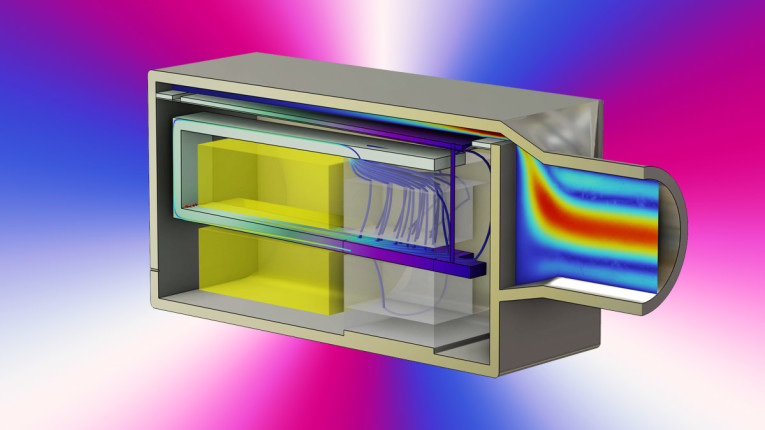
DC Field Solutions — Let’s first look at the DC solutions generated by the permanent magnet. Figure 4 shows the magnetic flux density (the B field) using streamlines (a) and its magnitude in slices (b). This DC magnetic field imposes Maxwell stresses on the armature, resulting in a static displacement of the armature and other moving components that are connected to it.
As seen in Figure 5, the portion of the armature sitting inside the air gap experiences the strongest traction (a), with a net force pointing upward, which pulls the solids so that they move upward (b). Note that a scale factor of 150 is applied to the deformation plot for visualization purposes.
The structural deformation directly affects the air-domain geometry, and this change is captured by the moving mesh functionality. Figure 6 shows a close-up of the original mesh when the armature is at rest (a) and the deformed mesh when it is actuated by the static magnetic force (b). A scale factor of 25 is used here for showing the deformation. Note that the magnetic field is solved in this deformed geometry, which, together with the DC magnetic field and static solid displacement, serves as the linearization point for the frequency-domain perturbation analysis.
Frequency-Domain Solutions — Now let’s look at the harmonic perturbation solutions on top of the DC bias. The study sweeps over a wide frequency range from 100Hz to 20kHz, and a plot of the maximum vertical deflection versus frequency at an evaluating point (located at the edge of the arm, as indicated by a red dot in Figure 7a) gives a good picture of the transducer’s behavior in regard to the driving frequency (Figure 7b; the blue point marker in the curve indicates the frequencies being studied). Here, we see a maximum displacement of 16µm at 2800Hz and two smaller peaks at 6300Hz and 14,000Hz. The vertical displacement field in all moving parts is depicted for 100Hz (a), 2800Hz (b), and 20kHz (c) in Figure 8, which shows that higher-order modes are excited in the diaphragm for higher frequencies (the displacement is exaggerated).
The effect of the resonance is also clearly seen in the electric impedance plot of the coil, as illustrated in Figure 10. The two solid lines show the absolute value of the coil impedance (blue) and its phase (red) calculated from our full multiphysics model.
After the resonance frequency, the inductance of the voice coil starts playing a more important role, resulting in a continued increase in the coil impedance. Here, we also include the published data (the two dashed lines) obtained from the lumped model by René Christensen of Acculution A/S, a modeling and simulation consultancy [4] for comparison. There is good agreement up to a frequency where the lumped model is not applicable anymore.
While the location of the resonance matches well, we see the biggest difference in the magnitude around the resonance. This is expected because the full FEM model includes (and a lumped model does not) the effect of the geometry change (in both the solid and fluid domains), which is the strongest around the resonance. Moreover, the magnitude at the resonance is solely controlled by damping. A slight difference in the damping description can result in quite notable discrepancy in the magnitude, and that is why one should be careful in comparing the response at and near the resonance.
Finally, let’s look at the acoustic response. The three images in Figure 11 show the sound pressure level at 100Hz (a), 2800Hz (b), and 20kHz (c), respectively. We can see that the sound pressure level is pretty evenly distributed on the cross section of the spout for all frequencies, and a maximum value of 142dB is obtained on the outlet at 2800Hz.
Figure 12 presents the sound pressure level received by the microphone that is used to measure the coupler response (Figure 2). The three resonances we see here coincide with those indicated in the displacement response curve shown in Figure 7. The plot also includes the results predicted from Christensen’s lumped model (red curve). Again, the agreement is quite good.
Now, we have discussed how to conduct a full electrovibroacoustic simulation of a balanced armature transducer. The analysis combines the electromagnetic field with structural vibrations and acoustic radiation, including the interplay between the multiple physical phenomena. A moving mesh is used to model the back EMF so that the varying reluctance of the air gap in the magnetic circuit is captured. The frequency-domain study gives detailed information for understanding and evaluating the performance of the driver undergoing small perturbations, which is important in the development of this type of transducer. The detailed model presented here can be used in an optimization analysis for innovative designs. aX
References
[1] Balanced Armature Transducer - Frequency Domain Analysis, COMSOL, www.comsol.com/model/balanced-armature-transducer-frequency-domain-analysis-61741
[2] M.R. Bai, B.C. You, Y.Y. Lo, “Electroacoustic analysis, design, and implementation of a small balanced armature speaker,” Journal of the Acoustical Society of America, Vol. 136, No. 5, pp. 2554–2560, 2014.
[3] J. Jensen, “Nonlinear Distortion Mechanisms and Efficiency of Miniature Balanced Armature Loudspeaker,” PhD thesis, DTU Electrical Engineering, 2014.
[4] R. Christensen, “Lumped Element Modeling of Transducers,” audioXpress, March 2023.
[5] M. Herring Jensen, “Full Multiphysics Electro-Vibroacoustic Analysis of a Balanced Armature Transducer,” INTER-NOISE and NOISE-CON Congress and Conference Proceedings (Inter-Noise 2022), Institute of Noise Control Engineering, pp. 1685–1691, 2022, www.ingentaconnect.com/contentone/ince/incecp/2023/00000265/00000006/art00078
[6] M. Herring Jensen, “Theory of Thermoviscous Acoustics: Thermal and Viscous Losses,” COMSOL, 2014, www.comsol.com/blogs/theory-of-thermoviscous-acoustics-thermal-and-viscous-losses
[7] R. Kampinga, “Viscothermal Acoustics Using Finite Elements Analysis Tools for Engineers,” PhD thesis, University of Twente, the Netherlands, 2010.
[8] M.R. Stinson, “The propagation of plane sound waves in narrow and wide circular tubes, and generalization to uniform tubes of arbitrary cross-sectional shapes,” Journal of the Acoustical Society of America, Vol. 89, p. 550, 1990.
[9] H. Tijdeman, “On the propagation of sound waves in cylindrical tubes,” Journal of Sound and Vibration, Vol. 39, p. 1, 1975.
[10] J. Huang, “Modeling Speaker Drivers: Which Coupling to Use,” COMSOL, 2022, www.comsol.com/blogs/modeling-speaker-drivers-which-coupling-feature-to-use
[11] IEC 60318-4:2010, Electroacoustics – Simulators of human head and ear, Part 4: Occluded-ear simulator for the measurement of earphones coupled to the ear by means of ear inserts, IEC, edition 1.0, 2010.
[12] Generic 711 Coupler — An Occluded Ear-Canal Simulator, COMSOL tutorial model, www.comsol.com/model/generic-711-coupler-8212-an-occluded-ear-canal-simulator-12227
[13] Transfer Matrix of a Tube and Coupler Measurement Setup, COMSOL, www.comsol.com/model/transfer-matrix-of-a-tube-and-coupler-measurement-setup-104291
This article was originally published in audioXpress, June 2024