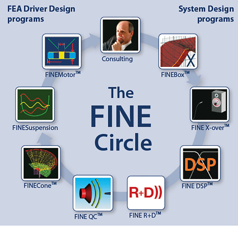
However, I’ve been impressed that Peter Larsen, over the years, has produced a group of programs and measurement hardware that accomplished all the various tasks required for a complete system design, the transducers, the enclosures, and passive crossover designs. His company, Loudsoft refers to this collection of hardware and software as the “FINE Circle” of design. The FINE Circle (Figure 1) includes the FINE R+D analyzer, FINEMotor, FINESuspension, and FINE Cone transducer software, and FINEBox enclosure design software, FINE X-over, and FINE DSP and network design software.
Given all this, I asked Peter to develop a tutorial for the design of a complete loudspeaker from transducer to final product. The target design will be a two-way speaker with a 6.5” woofer and a 1” dome tweeter. The following content was contributed by Peter Larsen.
Vance Dickason - Voice Coil editor.
The basic two-way Design Target for this tutorial is:
18-liter bass reflex box
Two-way design
6.5” woofer
1” dome tweeter
Frequency range: ~40Hz-30kHz
For the 6.5” woofer design, the following programs were utilized:
FINEBox initial simulation to define target Thiele-Small (T-S) data
FINECone Acoustical Cone and initial surround design
FINEMotor Motor Design
FINESuspension Design of surround and spider
FINE R+D analyzer for confirming woofer measurements
FINEBox Initial Simulation to Define Target Thiele-Small Data
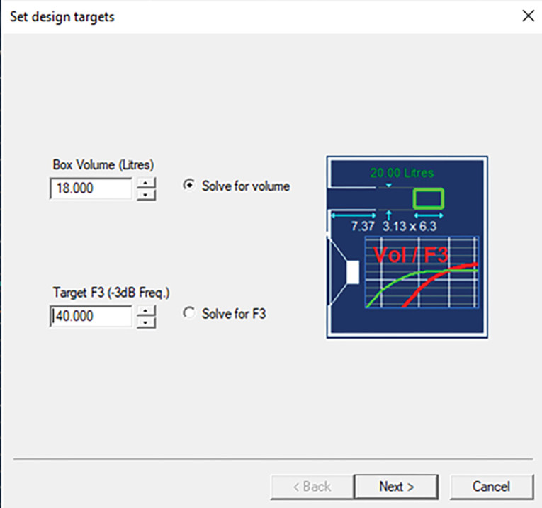
After starting FINEBox, I selected the ”Inverse FINEBox” program. As a design target, I input 18 liters and ”Solve for Volume,” as shown in Figure 2. From the drop-down list of default drivers in all sizes, I selected “165mm_6.5in typ.” Now we have enough data to start box simulations. The target T-S parameters are shown in Figure 3. The result of the initial simulation produced the brown dashed curve #1 shown in Figure 3. It gives ~98dB SPL with a -3db point at 50Hz, with 5.9V/4.33W input for getting Xmax (~3mm).
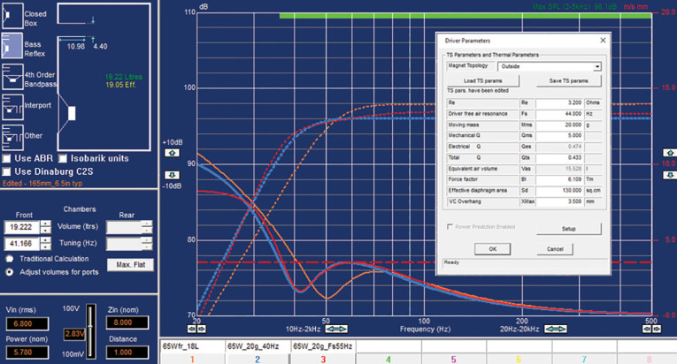
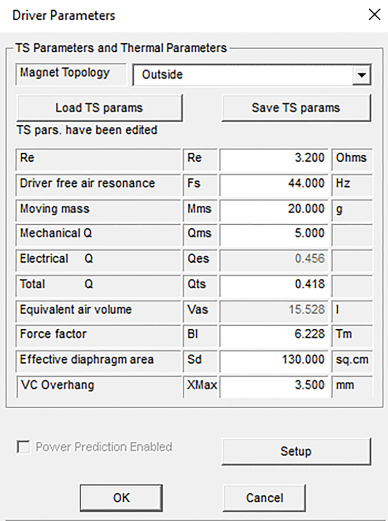
To reach the low-frequency target, we needed more moving mass. After increasing the moving mass to 20g and slightly increasing Xmax, I ran the Inverse FINEBox again, this time optimizing for F3=40Hz. This is shown as the blue dashed curve #2, which has -3dB at 40Hz. The target T-S data is shown in the grey window of Figure 4.
The red curve #3 shown in Figure 3 is a version with higher Fs, tuned slightly lower for reducing voice coil travel below 40Hz (see the solid red curve, lower left). The slight downward slope toward 40Hz helps to get a flat response in a room with wall and floor reflections (room gain from boundary loading).
Cone/Surround Design
In this next step I used FINECone to design the 6.5” cone, surround, and dust cap. After first selecting the Geometry Modeler, I then chose the Curvilinear Cone Woofer template, shown in Figure 5. Here we can simply insert the dimensions we want, while watching the actual geometry be continuously updated at left.
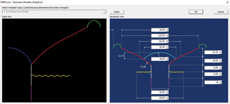
My 6.5” frame has a clamping ID of 143mm. Setting 10mm as initial surround diameter, the cone diameter then should be set to 123mm. After choosing a deep curvilinear cone, I specified a small and tall dust cap, for preventing dust cap break-up following my previous experiences. The Finite Element Model (FEM) will be automatically created from the Geometry Modeler.
FINECone automatically assigned typical values for the thickness of the cone, the surround, and the dust cap. In addition, the cone and dust cap materials were defined as DKM N-paper. The surround was a typical rubber type chosen from the database, plus a typical cotton spider with medium stiffness. Figure 6 depicts the calculated 0°/30°/60° frequency response of the 6.5” woofer with the given dimensions and materials.
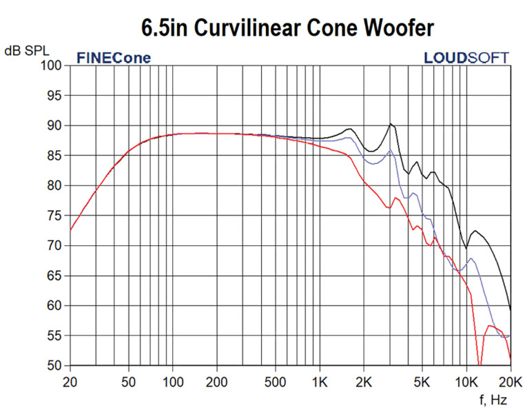
The calculated frequency response is not flat and has a couple of peaks ~1700Hz and ~3100Hz. At 1739Hz, the cone edge and inside surround edge bends down and almost in opposite phase of the cone. Figure 7 shows the calculated displacement at the 3039 mode, which is the first cone break-up mode in the outer part of the cone.
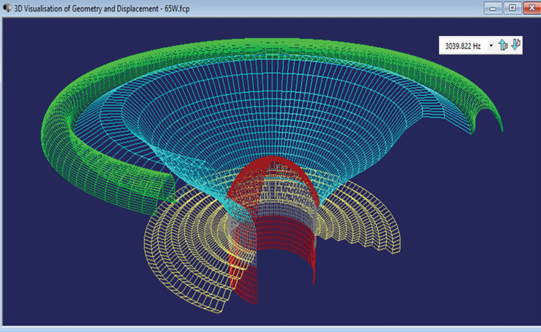
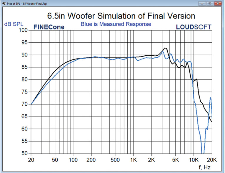
Figure 8 shows the final response (black curve) of the 6.5” woofer with the optimized cone and the surround plus dust cap. To suppress the cone/surround mode at 1739Hz, the surround thickness was increased from 0.35mm to 0.6mm. This was more effective than a thicker cone edge. In addition, the cone material was selected from the database as a talc-filled PP cone with high damping. The new response, illustrated in Figure 8, is now fairly flat up to the 3039Hz cone mode. The blue curve is the measured response of the actual 6.5” woofer using the FINE R+D analyzer. The calculated FINECone response is quite close to the measured results.
6.5” Woofer Motor Design
The initial FINEMotor simulation uses a 90mm×45mm×15mm Y30 ferrite magnet and cone/surround/dust cap mass from FINECone. In the Direct FEM window, which performs the magnetic Finite Element calculation, a 3mm bumped back plate was chosen, and the Bl(x) curve becomes symmetric after extending the pole piece by 3mm. However, the Bl is still lower than the target
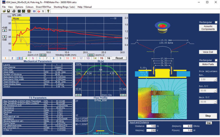
To get high Bl in a tight air gap, I chose a one-layer edge-wound voice coil. After focusing the B-flux with undercuts below and above the top plate, we get a nice solution, which is close to the target. However, the Qts=0.47 is still too high. Figure 9 depicts the final solution (#3), using a larger 90mm×45mm×20mm Y30 magnet, where no bump is necessary due to the thicker magnet.
Now let’s look at the voice coil induction Le(x).
Figure 10 displays the screen for Shorting Rings and Caps/Le(x) in FINEMotor, where we can insert rings in various places and in different materials and calculate the voice coil induction le(x) using the FEA engine. A standard copper ring under the top plate will lower Le(x), but it is most effective at low voice coil positions (negative x).
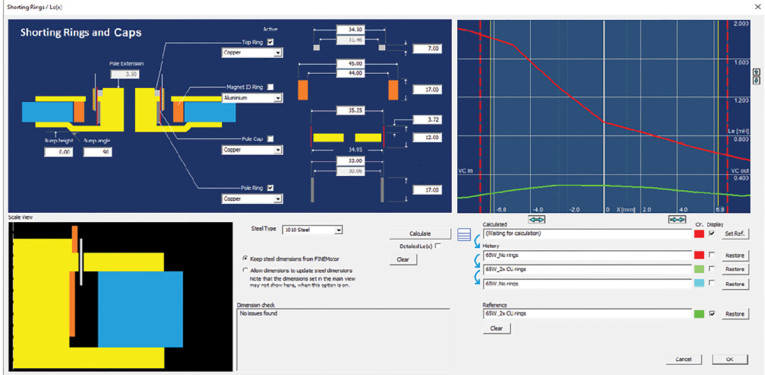
To prevent DC-offset while playing, the Le(x) curve must be symmetric around the Y-axis, which is seldom possible using only one ring. In Figure 10, I have therefore inserted two copper rings below and above the top plate. They are different in thickness and length, causing the resulting Le(x) curve (green) to be quite symmetric. The red curve shows Le(x) without any rings, and the improvement of Le(x) is remarkable.
Fine Tuning the Suspension Design
From FINECone, we received a preliminary design for the surround. Next, I optimized the large signal parameters in the nonlinear domain using FINESuspension. I began with Half-Roll Template 1 and input the dimensions I already knew — the roll diameter (10mm) and 0.6mm thickness, and clamping ID 143mm, as shown in Figure 11. The Km(x) stiffness curve was calculated using Non-Linear FEA and is nicely U-shaped, however not symmetric (observed from the dashed mirror curve).
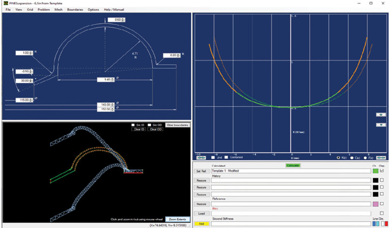
Since the previous curve showed less upward movement capability, I compensated by moving the cone flange down. The calculated Km(x) curve was now fully symmetric. The green range indicated the usable ±5.5mm range (per IEC62458), which is OK. This is shown as the lower curve in Figure 12. I also used FINESuspension to calculate a suitable spider, as shown in Figure 12. Using Spider Template 4, I input the known dimensions of the inner diameter (ID) and outer diameter (OD). Playing with the wavelength, I found 5.7mm (between wave tops) produced a spider with a nice flat area close to the voice coil. That would be covered with stiff glue, which I define by the green fixture lines.
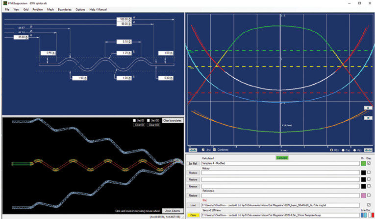
The calculated Km(x) curve is good, but not symmetric because the spider has less downward movement capability. I chose to compensate for that by moving the voice coil flange up and the outside down. The Km(x) spider curve was now symmetric (the lower curve shown in Figure 11). The previous surround Km(x) curve was imported as the middle blue curve.
Above that, the Km(x) of the combined surround + Spider was shown as the Red/White curve, having a working range of ±5mm (per IEC62458). Ideally, this should be comparable to the operating range of Bl(x). For this reason, I imported Bl(x) from FINEMotor as the upper curve. The green range was almost the same, ensuring enough stiffness above Xmax. This provides very high stability. Stay tuned for Part 2! VC
Read Part 2 of this Tutorial here.
Read Part 3 of this Tutorial here.
This article was originally published in Voice Coil, July 2023.