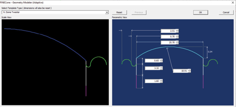
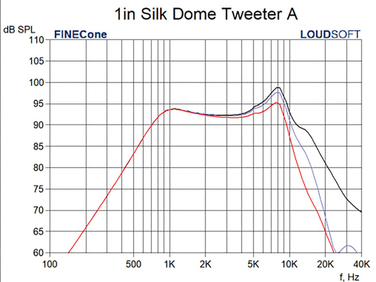
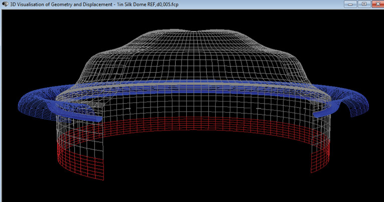
Using the Loudsoft FINECone diaphragm simulation software, I have selected the Dome template shown in Figure 1 and specified the typical dimensions for a 26mm silk dome with surround. The result of the first FINECone simulation, tweeter A is shown in Figure 2 for on-axis and 30°/60° off-axis responses. The initial simulation will automatically use suitable parameters by default and can therefore be trusted. The response is gradually peaking up to 8kHz due to break-up starting around 5kHz. This is shown in Figure 3, which displays the first-order break-up at 5110Hz where the dome starts bending from the edge.
From other simulations, we know that a higher profile has increased stiffness vertically. Therefore, let us examine a higher dome profile. The calculated 0°/30° (black/blue) frequency response of the higher dome tweeter is shown in Figure 4. Now the break-up products are shifted up, starting from ~10kHz. The dome was split into two parts, where the ring closest to the voice coil’s edge is stiffened by glue. The red response is an actual measurement of this naked dome (i.e., without any other face plate or similar). Apart from the actual sample having more damping at ~1100Hz, the red curve is remarkably close to the simulated response! The dip at 7kHz comes from the imperfectly woven silk/fabric material.
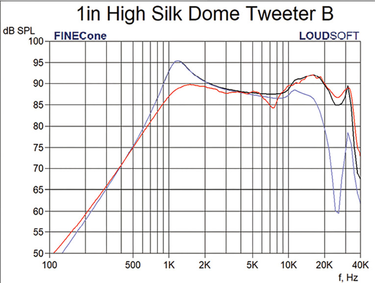
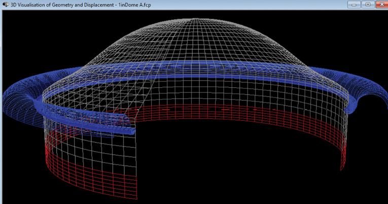
Figure 5 depicts high-order break-up at 15189Hz of the higher profile dome. Interestingly, this break-up behavior is normal for soft dome tweeters, which have early break-up due to the soft (silk) material. However, these break-up products are usually well controlled due to the high damping with the typical soft dome materials like this pre-coated dome.
Since the soft dome tweeters depend so much on damping, we would want to apply as much as possible. The downside is lower sound pressure level (SPL) caused by the increased mass and maybe loss of high frequencies. The damping glue used to be applied by a brush and therefore difficult to add evenly. Today’s pre-coated “silk” materials do not suffer from this problem and usually have enough damping.
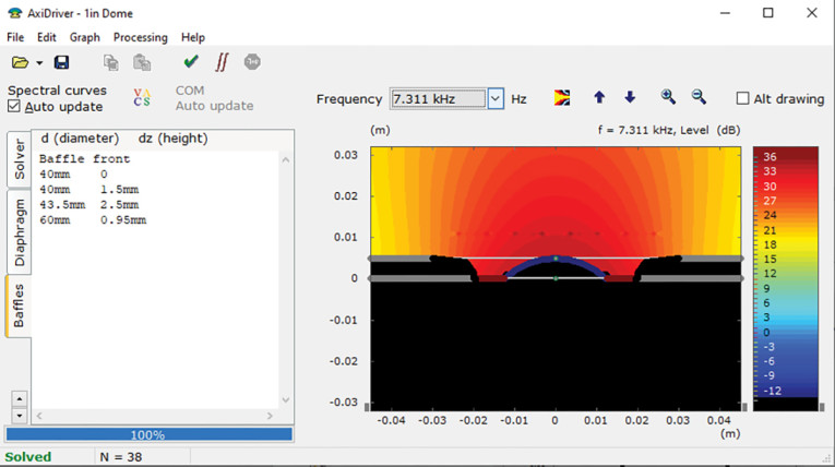
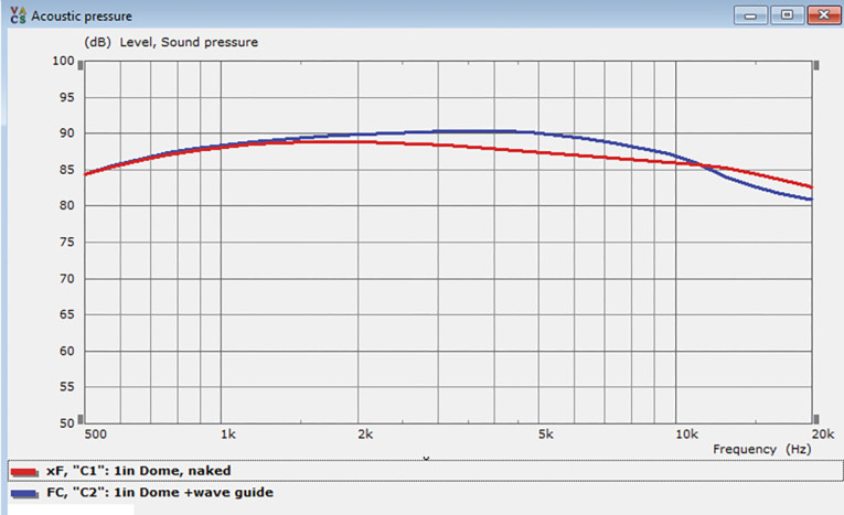
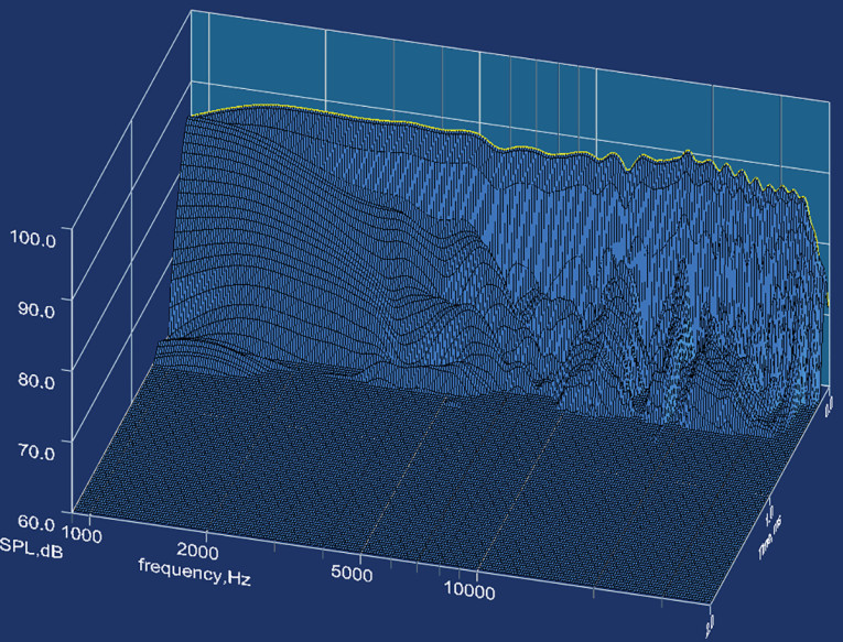
One way to achieve a flatter response is by adding a small wave guide. A wave guide/horn only works at medium frequencies and may therefore help by filling out the lower area below break-up, in this case ~2kHz to 10kHz. It is possible to simulate the wave guide effect on the frequency response using BEM software. Figure 6 illustrates Axidriver and VACS (Randteam.de) used to simulate a small wave guide for this purpose. This effect is shown in Figure 7, where the frequencies from ~1.5kHz to 10kHz will be amplified, which will smoothen the total frequency response. The cumulative waterfall plot from FINE R+D is shown in Figure 8. This is well-behaved beyond 1mS. There are a couple of decaying resonances above 10kHz, which may be damped with more coating glue.
Now it is time to design a suitable motor for this dome tweeter. After inserting the dimensions and mass from FINECone into FINEMotor, I have optimized a ferrite magnet motor as displayed in Figure 9. The top plate thickness is 2.5mm, which works well in the Direct FEM mode. However, in this case, I have focused the gap flux slightly better by inserting chamfers on the pole and top plate as indicated lower right.
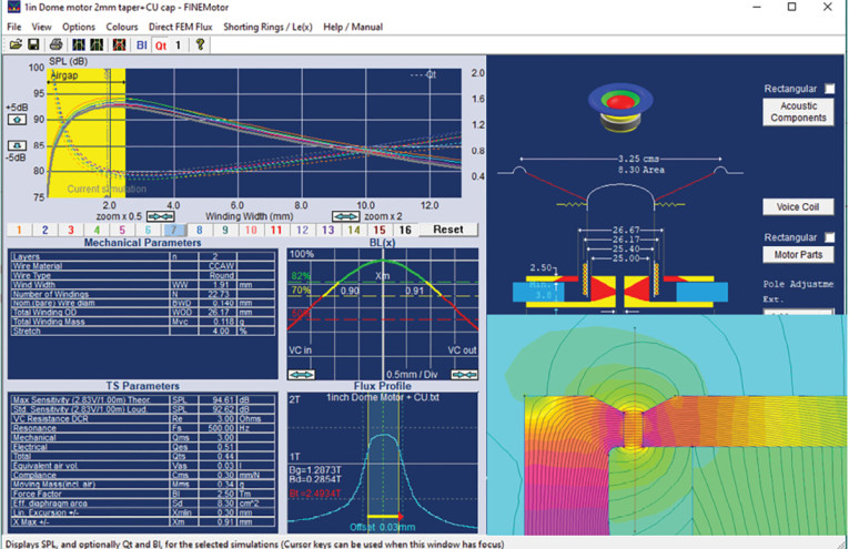
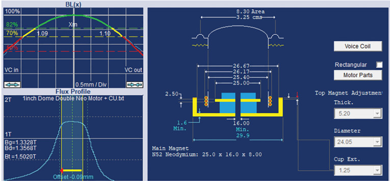
Note that BL(x) curve is fully symmetrical. The green working range for minimum 82% BL is ±0.90mm, which is much more than needed for this 1” dome tweeter. The pole is close to saturation because it has a quite large 16mm through hole for good acoustical connection to the rear chamber, as shown in Figure 10. The active neodymium (neo) magnet ring becomes quite small with the large center hole. Therefore, I selected the high N52 neo grade, and a top neo magnet ring magnetized opposite to force some of the leaking flux back into the air gap. The resulting sensitivity is close to the ferrite motor. It is difficult to arrange the dimensions of the two neo magnets for getting a symmetric flux in the air gap, but the outer height of the magnet yoke/cup was increased by 1.25mm to help the flux above the top plate. The resulting BL(x) becomes quite symmetrical when the voice coil was offset by 0.09mm.
If even higher sensitivity is needed, I experimented with a large outside neodymium disk. This neo magnet is considerably larger and the cost will be higher. Figure 11 shows how the pole piece is now extremely saturated, which really sets the limit. Reducing the center hole diameter could potentially get even higher flux and sensitivity.
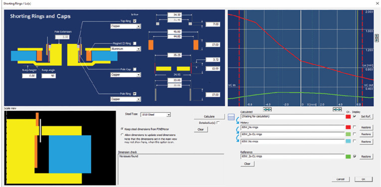
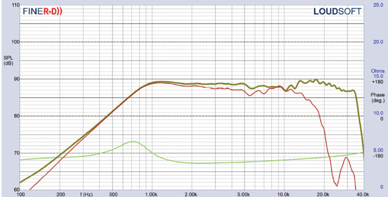
Figure 12 gives the final response of the 1” soft dome tweeter with ferrite magnet system. The on-axis response is very flat, and the 30° off-axis response is gently sloping down, which is very close to the target response.
Next Article
In Part 3 of this article series, I will go through the development of a two-way passive crossover network for the 6.5” woofer and 1” silk dome. VC
Read Part 1 of this Tutorial here.
Read Part 3 of this Tutorial here.
This article was originally published in Voice Coil, August 2023.