
The first two parts of this article series demonstrated the development of a 6.5” woofer and vented enclosure along with the high-frequency transducer, a 1” silk dome tweeter, as part of this Loudsoft simulation software system design tutorial. The final step in this system design tutorial is to develop an appropriate passive network design.
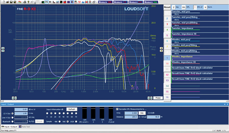
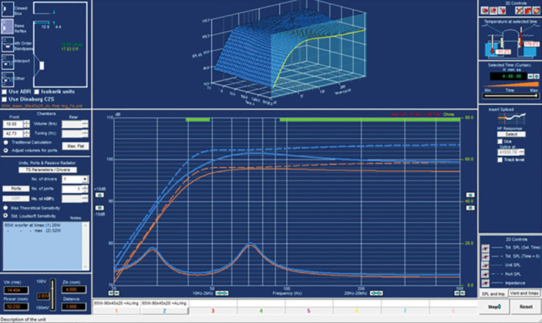
I began this process by placing the woofer and tweeter constructed from the data developed in the first two articles in the cabinet and then measuring the 0° on-axis and the 30° and 60° off-axis frequency response and phase and impedance with phase using the Loudsoft FINE R+D FFT analyzer (Figure 1). The phase responses are not shown.
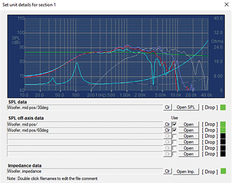
I started the system design in FINE X-over by dragging and dropping the measured responses directly from FINE R+D (Figure 2). Note that I placed the 30° off-axis response first, thereby optimizing that to the slightly sloping target (the green line shown in Figure 2). In FINE X-over, the woofer and the tweeter crossover sections will be optimized with individual targets.
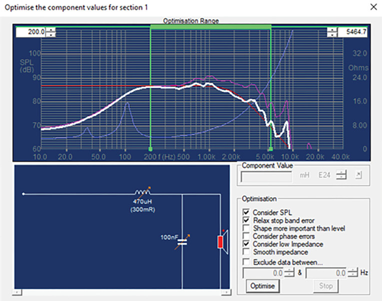
Starting with the woofer, (section 1) illustrated in Figure 3, I chose a simple second-order low-pass Butterworth filter. This will work well given the well-behaved woofer frequency response. Setting the cross-over frequency to 2kHz, we get a target low-pass Butterworth curve (red). After optimizing, the white response is close to the target. The “Consider low impedance” was set for avoiding the impedance dropping below the standard 3.2Ω for a 4Ω nominal impedance. We also have the option of inserting more components for higher-order networks, impedance compensation, etc. later.
For the tweeter section shown in Figure 4, I chose a third-order high-pass network by setting a fourth-order target for matching the measured response. I also selected a series resistor for attenuation. The component values are automatically determined by the optimizer, including the resistor.
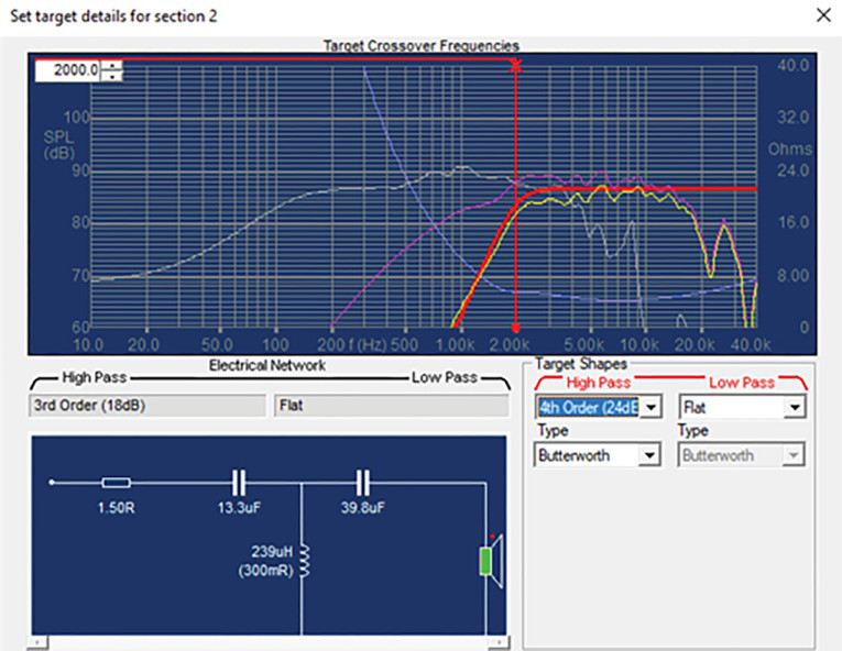
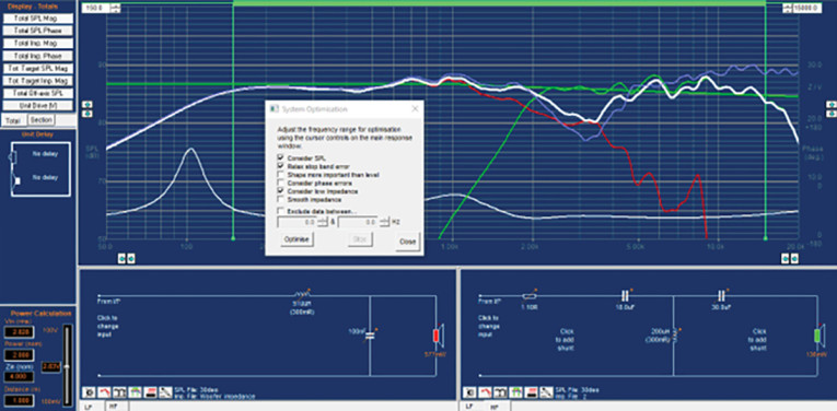
Figure 5 shows the total response with optimized woofer and tweeter sections. The response is not flat, despite the optimized sections. Therefore, I will optimize the total system response next, including impedance, which guarantees the minimum impedance of 3.2Ω is always retained.
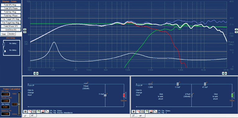
The total optimized 30° and 0° responses plus impedance are displayed in Figure 6. The white 30° response was optimized to the green slightly down-sloping target. Interestingly, the actual cross-over frequency has moved up! This optimized response is quite flat and useable.
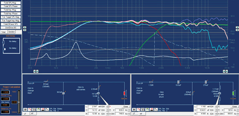
However, in Figure 7 I have inserted some extra components, in the form of two series RLC circuits, placed in parallel with the woofer and tweeter. This further made the response flatter. The first RLC is in the woofer section at 838Hz and the second in the tweeter section at 5814Hz. For both sections, levels, bandwidth, and frequency were tuned using the mouse wheel. The low end was added as a spliced near-field response (brown).
The power compression at continuous high-power input is calculated in Figure 8. Using the previous FINEMotor data, the power compression was calculated with an input giving Xmax for the woofer (brown 1). Increasing to maximum power input caused approximately 4dB power compression causing a magnet temperature of 51.2°C, and a voice coil temperature of 179°C (blue). This sounds very high but is much lower for real music, which has an effective duty-cycle below 30% or lower.
Alternative DSP Crossover with Boost
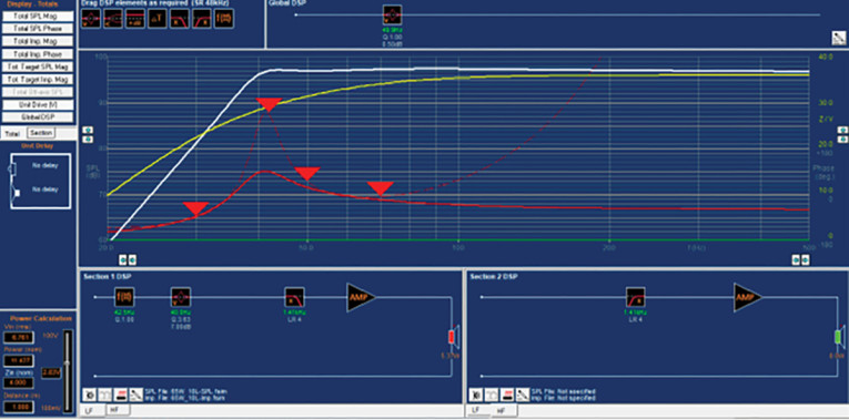
As an alternative, I imported the measured speaker responses into the Digital X-over software FINE DSP, depicted in Figure 9. The white curve was optimized for the green target using DSP with several Biquads making the curve really close to the target. In addition, the dashed white phase response was also much smoother.

We could also use the DSP in a smart way by applying a large boost at the tuning frequency Fb of the vented system, where the woofer cone travel is minimum. This is calculated using FINEBox, shown in Figure 10, where the original 18-liter response is shown as the brown dashed curve. Using the advanced “Inverse FINEBox” feature I found that a smaller 10-liter box can produce the same low-frequency extension as the original 18 liter, by using DSP boost and high-pass filter. This is shown as the blue curve, which here is set to show the possible low frequency extension possible with DSP (=the flat “knee” around 40Hz). Next, I will show how this is done in FINE DSP.
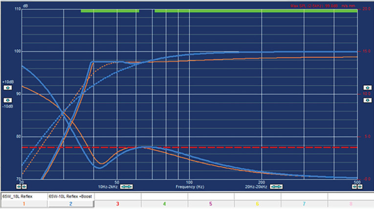
Figure 11 illustrates the 10-liter system with DSP boost and low frequency cut (white). The final boosted input voltage is shown as the solid red line. I had earlier exported the Maximum Voltage for (obtaining) Xmax from FINEBox, which is displayed as the dashed red line. The potential for a boost at 42Hz is large, and not even fully used in this example. However, with an increasing boost we also need to increase the level above and below 42Hz to keep a flat response, and that would quickly hit the maximum allowable voltage. The yellow curve is without a boost for comparison. In addition to the low-frequency extension we also get a little more SPL.
The DSP (SPL, Q, dB) settings can be exported to any DSP hardware either directly or as coefficients. The user can therefore choose an inexpensive MiniDSP or similar or a more advanced state-of-the-art DSP such as Danville Signal’s Nexus or one of the DSP processors from Marani Pro Audio.
In Conclusion
I have now been through the FINE Circle, starting with FINEBox and using the three FEA programs: FINEMotor, FINECone, and FINESuspension to develop drivers. Then I measured them with FINE R+D and designed a crossover with FINE X-over and FINE DSP. Later, when drivers and systems are being produced, both can be automatically tested with FINE QC, including the best in industry Rub & Buzz testing. For more information about all the Loudsoft FINE Circle of programs for complete transducer and system design, as well as the Loudsoft FINE R+D analyzer hardware and FINE QC hardware, visit www.loudsoft.com. VC
Read Part 1 of this Tutorial here.
Read Part 2 of this Tutorial here.
This article was originally published in Voice Coil, September 2023.