Dayton Audio sent a pair of new shallow-mount home/car audio subwoofers, the 10” LS10-44 and the 12” LS12-44. One of the most pervasive trends in loudspeaker design over the last few years is to create speakers that are heard, but not necessarily seen. While the public once mostly wanted ostentatious off-wall speakers that dominated a room, the market today for in-wall, on-wall, and in-ceiling speakers now constitute a large percentage of what is being manufactured.
One of the harder problems to solve is how to make subwoofers “disappear.” While there have been a lot of different solutions to in-wall subwoofers, getting large diameter woofers to fit in a 4” deep space has been a challenge for transducer engineers. However, the market has produced a variety of clever methods to achieve this goal. Shallow mounting is also very desirable in car audio, so these woofers appeal to both markets. Two of these under 4” deep subwoofers appeared in previous Voice Coil issues — the SB Acoustics SW26DAC76-8 (September 2009) and the Peerless P85028 (September 2010).
Dayton Audio’s LS10 and LS12
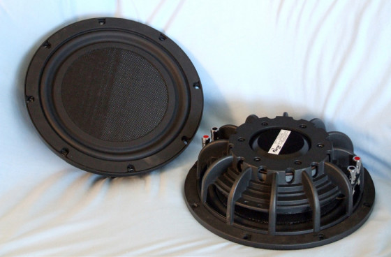
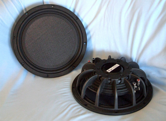
This month, Dayton Audio sent me two shallow-mount subwoofers, the LS10 (see Photo 1) and the LS12 (see Photo 2). Both subwoofers are less than 4” deep. Since these are 10” and 12” versions of the same concept, I’m going to analyze the Dayton Audio LS10/12 together rather than separately.
Measured from the bottom of the frame mounting surface to the back of the motor system, the 10” LS10 is only 3.3” (84.5 mm) deep, while the LS12 is only slightly bigger at 3.9” (98.5 mm) deep, making both drivers relatively easy to mount between two 2” × 4” studs in a standard framed wall. This is accomplished by using a standard ferrite motor mounted within the driver frame. In terms of features, both subwoofers are built on similar 12-spoke proprietary cast-metal frames. While the frames lack venting below the spider mounting shelf, they do have 12 10 × 15 mm vent holes in back of the frame, where you would normally mount a front plate. These holes enable air to circulate over the front plate and magnet and exhaust out the rear of the frame. The motor assembly’s T-yoke is bolted (and presumably also glued) to the frame using six bolts.
Both cone assemblies consist of an extremely stiff flat honeycomb fiberglass cone. Both flat cones are coupled to the voice coil neck joint with short flat profile conical cones—3” diameter for the LS-10 and 4” in diameter for the LS-12, both vented. (The formers are also vented.) Suspending this very stiff flat cone is a unique “S” shaped “balanced roll” nitrile-butadiene rubber (NBR) surround. Both devices use the same damper assembly that includes a phenolic mounting ring and a 6” diameter flat treated cloth spider. Driving all this are 50 mm (2”) diameter dual 4-Ω voice coils wound with round copper wire on a non-conducting Kapton former with the tandem voice coil lead wires stitched into the spider. Topping off the features are dual shorting rings and a pole extension. Voice coil lead wires are terminated to chrome-plated, color-coded terminals on opposite sides of the frame.
I began analysis of these shallow-mount Dayton Audio subwoofers using the LinearX LMS analyzer and VIBox to create both voltage and admittance (current) curves with the driver clamped to a rigid test fixture in free air at 1, 3, 6, 10, 15, 20, and 30 V. I no longer use a single added mass measurement and instead use actual measured mass. LEAP 5 was able to adequately curve fit all the different voltage curves, so I post-processed 12 550-point stepped sine wave sweeps for each of the Dayton subwoofer samples and divided the voltage curves by the current curves (admittance) to derive the impedance curves.
I used the LMS calculation method to derive the phase and, along with the accompanying voltage curves, I imported the data to the LEAP 5 Enclosure Shop software. Since the majority of the Thiele-Small (T-S) data provided by OEM manufacturers is produced using either a standard method or the LEAP 4 TSL model, I additionally created a LEAP 4 TSL model using the 1-V free-air curves. I selected the complete data set, the LTD model’s multiple voltage impedance curves, and the TSL model’s 1-V impedance curve in the transducer derivation menu in LEAP 5 and created the parameters for the computer box simulations.
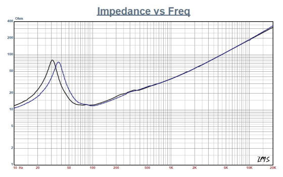
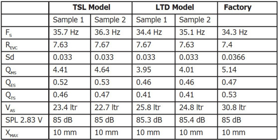
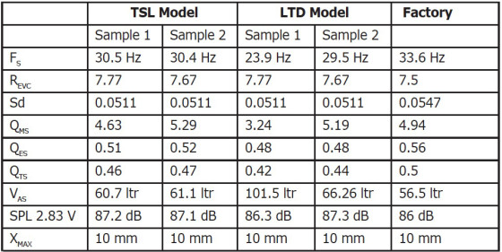
Please note that both voice coils of each driver are wired in series for these tests. Figure 1 shows the 1-V free-air impedance curves for the LS-10/LS-12. Table 1 and Table 2 compare the LEAP 5 LTD and TSL data and factory parameters for both sets of samples.
The LS-10/LS-12’s LEAP parameter calculation results both correlated well with the factory T-S parameters, with the biggest discrepancy being the Sd calculation, which was less conservative than mine. The Sd in Voice Coil’s test bench analysis is calculated from the woofer cone assembly diameter extending from the center of the surround to the opposite center of the surround. This is intended to represent the approximate contribution of the surround radiation to the overall sound pressure level (SPL). Regardless, with close agreement between my data and that published by Dayton Audio, I proceeded to put together computer enclosure simulations using the LEAP LTD parameters for the LS-10 and the LS-12 Sample 1 drivers.
I set up closed-box simulations for both woofers that would result in a QTS = 0.7. This resulted in a 0.45-ft3 sealed box with 50% fiberglass fill material for the LS-10, and a 1.2-ft3 enclosure also with 50% fiberglass fill material for the LS-12. Taking a preliminary look at the results, F3 was 55 Hz for the LS-10 and 48 Hz for the LS-12. If the application were a modest-sized car compartment (120 ft3), then the acoustic “lift” from the closed field would provide a response below 20 Hz (see Figure 2). However, in a home-audio environment, a lower F3 would be a good goal. Rather than try the poorly damped vented alignments that would result from the relatively high QTS of both Dayton subwoofers, I augmented the response with a large series capacitor.
This technique was published in an Audio Engineering Society (AES) paper titled “Closed-Box Loudspeaker with a Series Capacitor” by Neville Thiele (Journal of the Audio Engineering Society, July 2010) and was republished in the November 2012 issue of Voice Coil magazine. After some quick empirical “cut and try,” I found that a 200-μF capacitor provided satisfactory results for both subwoofers.
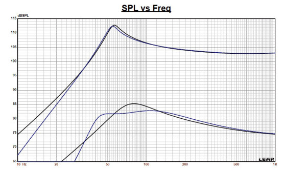
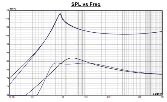
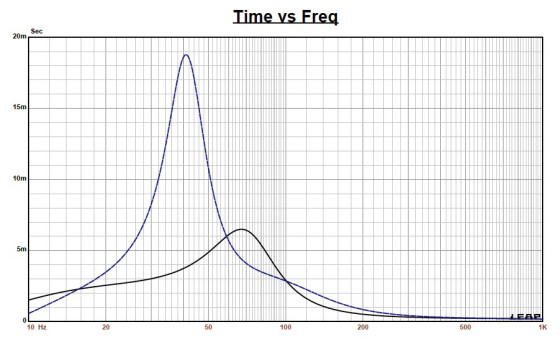
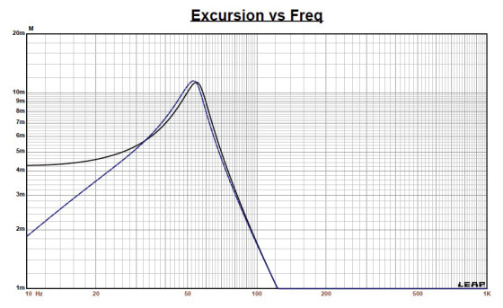
Figure 3 shows the outcome for the Dayton Audio LS-10. Figure 4 shows the LS-12 in the two sealed boxes at 2.83 V, and in the same two boxes with the 200-μF series capacitor. These simulations were also done at a voltage level sufficiently high enough to increase cone excursion to 11.5 mm for both the LS-10 and the LS-12 (XMAX + 15%). For the LS-10, this generated a F3 frequency of 55 Hz with a box/driver QTC of 0.69 in the 0.45-ft3 sealed enclosure and –3 dB = 40 Hz (QTC = 1) for same enclosure with a 200-μF series capacitor. I increased the input voltage until the achieving 11.5-mm excursion point (120 V) produced an SPL of 113 dB, both with and without the series capacitor. Figure 5 and Figure 6 show the group delay and cone excursion curves for the LS-10, respectively.
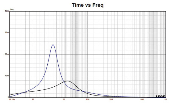
Looking at Figure 4, the LS-12 in the 1.2-ft3 sealed box simulation yielded an F3 = 48 Hz (QTC = 0.69). With the series 200-μF capacitor, the LS-12’s F3 lowered to 34 Hz (QTC = 0.92). Increasing the voltage input to both simulations until the maximum linear cone excursion was achieved produced 113 dB at 120 V for the sealed enclosure, again with and without the series capacitor Figure 7 shows the 2.83-V group delay curves.
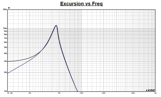
Figure 8 shows the 120-V excursion curves. Unfortunately, we had some scheduling conflicts as we approached the deadline on analyzing the LS-10 and the LS-12, so I weren't able to publish our usual Klippel analysis.
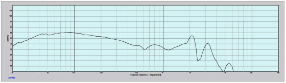
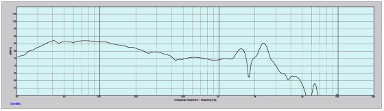
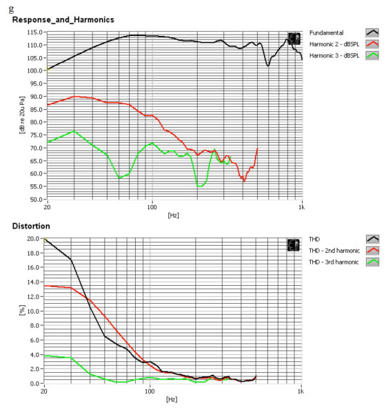
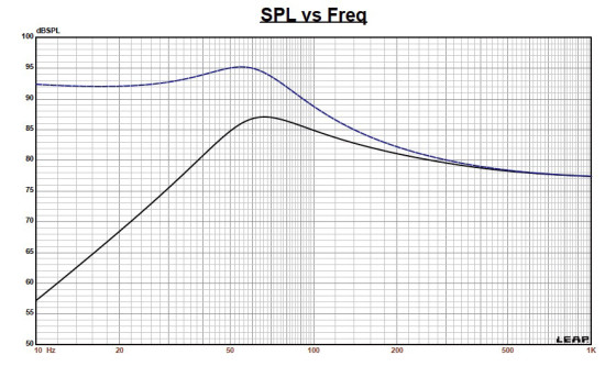
Even though this is a subwoofer and the driver would likely be crossed over in the vicinity of 100 Hz or lower, I generally like to take SPL data, as there is always the possibility for any subwoofer to fit into a more conventional three-way format with a crossover frequency in the 200-to-400-Hz range. I did try to measure the SPL on these subwoofers, but the levels were so far down at the lower range that I can measure in my test environment I decided instead just to republish Dayton Audio’s SPL for these drivers, as seen in Figure 9 for the LS-10 and Figure 10 for the LS-12. For the remaining group of tests, I used the Listen SoundCheck analyzer, 0.25” SCM microphone and power supply (courtesy of Listen, Inc.) to measure distortion and generate time-frequency plots. For the distortion measurement, the LS-10 subwoofer was mounted rigidly in free-air, and the SPL set to 94 dB (21 V) at 1 m using a noise stimulus.
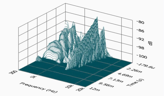
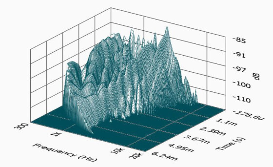
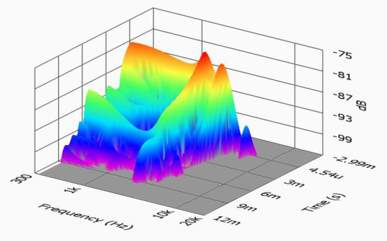
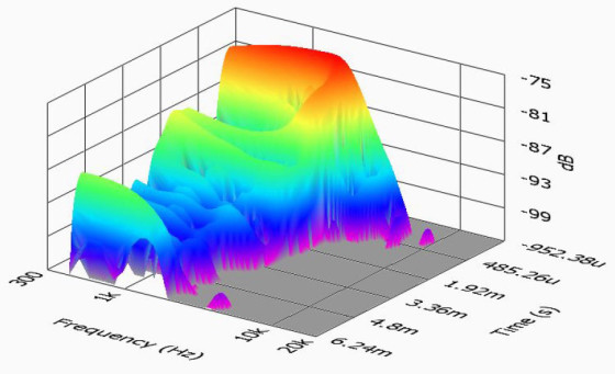
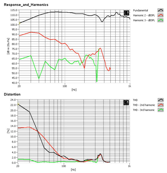
I measured the distortion with the Listen microphone placed 10 cm from the dust cap. This produced the distortion curves shown in Figure 11. I performed the same procedure on the LS-12, resulting in the distortion curve shown in Figure 12. I then used SoundCheck to get a 2.83 V/1 m impulse response for each driver and imported the data into Listen’s SoundMap Time/Frequency software. The resulting cumulative spectral decay (CSD) waterfall plots for the LS-10 and LS-12 are shown in Figure 13 and Figure 14, respectively., Figure 15 and Figure 16 show the Wigner-Ville (for its better low-frequency performance) plots for the LS-10 and the LS-12. It’s obvious from these graphs that the LS-10 and the LS-12 are best suited for subwoofer applications crossed over at 100 Hz or lower, which is exactly the application for which they are intended.
www.daytonaudio.com