
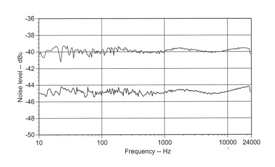
This figure shows the lower dynamic range of the swept frequency measurement. TrueRTA software
with 1/24-octave analysis and 10,000 point averaging.
Random Noise
The sound of rain on a metal roof, the sound of a waterfall, static between radio stations, and the “snow” on a TV screen not tuned to an active channel are all examples of random noise. Generally, these would not be useful for making measurements.
To be useful for measurements you need a known frequency spectrum: white, pink1, or other shape that has a known amplitude density — you hope it’s Gaussian (the bell-shaped curve) with a near-zero mean value and another item I will cover later. However, you can’t know what the next amplitude value is going to be. If you sampled the noise waveform for a lifetime you still wouldn’t be able to predict the next value with any degree of certainty. That’s because random noise is. . . random.
The other feature that makes the output signal of a random noise generator useful is stationarity. Without all the math, this simply means that the mean and mean-square amplitude values don’t change, in the statistical sense, with time.
In 1965 I did a study on the stationarity of laboratory random noise generators using long-time averaging (integration) of the mean and mean-square output voltages2.
I took data from three commonly available generators of that time: Allison Laboratories model 655, Brüel and Kjaer model 1402, and General Radio Company model 1390-A. My conclusion stated: “Within experimental limitations imposed by the measuring system, the noise sources evaluated were found to be sufficiently stationary for many laboratory uses.” In practice, this means that if I make a measurement today with a certain random noise generator and I make the same measurement tomorrow with the same generator, the results will be the same within a known percentage.
The Allison model was solid-state in an encapsulated module, so I have no knowledge of the circuit. The B&K used a pair of zener diodes for the noise generation in an otherwise all-vacuum-tube design, and the General Radio used a diode-connected triode in a magnetic field to generate the noise in an all-vacuum-tube circuit. I have no doubt that modern generators are as good as — if not better than - these vintage models.
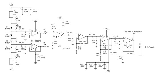
I have designed and built a prototype of a very good random noise generator, the TDL model 131. It is not in production because I suspect little sales interest — pseudorandom generators are more popular. You will see in the Applications section that random and pseudo-random (P-R) pink noise produce similar results. I have included the noise generation circuit diagram of the 131 as Figure 2.
Summing the noise voltages from the two zener diodes (D2 and D3) is required for equal positive and negative noise peaks. Random noise is also used for some types of encryption — coin toss simulators and the like — and it was used extensively for electrical and electromechanical measurements in the days before P-R generators.
Pseudo-Random Noise
Due to its popularity, much noise testing these days is done with P-R noise because it repeats, like a sine or square wave, yet it retains broadband. Because it repeats, it has a “line spectrum” rather than a continuous spectrum (like random noise). The “lines” are spaced in frequency equal to the reciprocal of the repetition time so the line spacing can be made to approach a continuous spectrum by lengthening the repetition time. But even for a repetition time of 200 ms, the lines are spaced only 5 Hz apart, which is adequate for many tests.
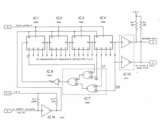
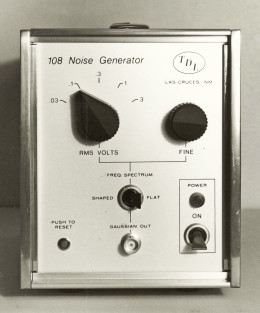
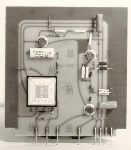
P-R noise is easily generated with shift registers, which became practical with the development of integrated circuit (IC) logic. I built P-R generators in the 1970s, first with RTL logic, and then with 7400-series TTL logic. Photo 1 shows one of these, the TDL model 108, and Figure 3 is its shift-register circuit diagram.
The model 108 used four 5-bit shift-registers (IC1-IC4) connected to generate a maximal-length P-R sequence of 1,048,575 bits (ones and zeroes) before repeating. With a 1 MHz clock, the sequence will repeat approximately once per second with a spectral line spacing of about 1Hz within the 50 kHz lowpass bandwidth. This illustrates another relationship that is part of the trade-off in designing P-R generators: the –3 dB bandwidth is equal to the clock frequency divided by the shift-register length. In this case: 1 MHz/20 = 50 kHz. This ratio has been found to give the best “fit” between the generator’s amplitude probability density and the desired Gaussian (bell-shaped) curve3, 4.
The 108-series enclosures were from
Buckeye Stamping Company;
they were very reasonably priced… then.
Output from the first and 16th flip-flops are exclusively- ORed (XOR), and this output is XORed with the XOR output from the 17th and 20th flip-flops in IC7. This output is inverted by IC8 to produce the feedback into the first flip-flop. This is one maximal-length, linear feedback arrangement for a 20-stage P-R register. Testing showed that this feedback produced a noise output with a flatter spectrum than any of the other possibilities for a 20-stage register. There are tables of maximal-length, P-R registers showing the length and feedback. I like the tables in Appendix C of this book5. But, as I found out with the 20-stage resistor, not all the table entries have a sufficiently flat frequency spectrum, so testing is required.
The remaining part of the generator consists of a level shifter circuit (for equal positive and negative peaks), an analog four-pole Butterworth lowpass filter (white noise output), and a “pink” lowpass filter for a spectrum with an equal energy per octave.
These days, the P-R sequence is perhaps easily generated with a microprocessor (μP). The TDL model 109 generator uses a Scenix - now Ubicom (meanwhile acquired by Qualcomm, www.qca.qualcomm.com) - SX28AC mP to simulate a 21-bit S-R clocked at 1 MHz. (The SX28AC runs at 25 MHz to clock the S-R at 1 MHz.)
This gives a bandwidth of about 50 kHz and a spectral line spacing of 0.5 Hz (a repetition time of two seconds)6. Figure 4 shows the pink noise spectra from a model 109 and a model 131. The P-R noise is perhaps a bit smoother, but there is not much difference.
Measurement Applications
1. An electronic filter’s amplitude response is easily measured because the broadband signal traces the response on the screen of a spectrum analyzer. Spectrum analysis software is readily available. I have a preference for TrueRTA7, which is a constant percentage bandwidth analyzer. If you prefer a constant bandwidth, take a look at Audiotester8.
Multi-Instrument9 offers both bandwidth options.

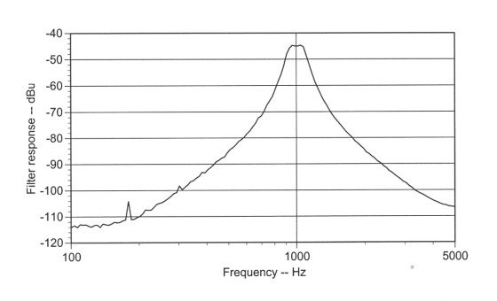
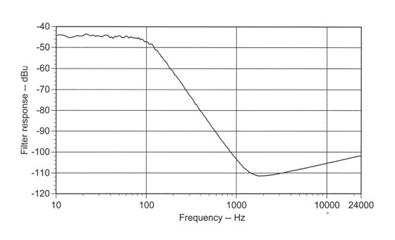
Figure 5 shows the measurement setup. Figures 6 and 7 show the responses for active bandpass and lowpass filters measured with pink random noise from a model 131, while Figures 8 and 9 show the responses measured with pink P-R noise from a model 109. P-R noise may produce a slightly smoother curve but the difference is small. To get a smooth curve the analysis program needs to be set to average a large number of points. (These four figures were produced with TrueRTA, 1/24-octave analysis and 10,000 point averaging).
You can also use this method to measure the response of amplifiers, but you need to observe one caution. The crest factor (peak voltage divided by the RMS value) is about 3.5 for both random and P-R noise, so be careful to not overdrive the amplifier. This is a peak-to-peak voltage of at least seven times the RMS. This caution would also apply if the filter has higher than unity gain.


2. In the early 1970s an East Coast company contacted TDL looking for a gated P-R noise generator. That is, they needed a generator that when commanded by an external trigger would turn on for a set time, then go off and wait for the next trigger. This company had a contract to seal abandoned coal mines and then demonstrate that the seal was airtight.
They intended to place several large loudspeakers in the mine before sealing it with the cables to the speakers embedded in the seal. Then they would send the “noise bursts” from the gated generator to the speakers through a large power amplifier. Using gated noise would allow their measuring equipment to average out the background noise from wind, bird song, traffic, and so on.
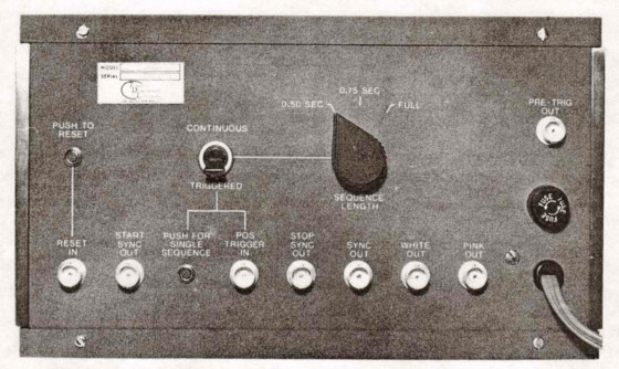
on the rear panel. This model was supplied in an adaptor for rack mounting.

The connectors and guides for
the plug-in circuit boards were part
of the Buckeye enclosure system.
To meet their need, we designed and built several model 108-M4 generators (see Photos 2 and 3). All the 108-series generators were designed around a group of uniform-size plug-in circuit boards (see Photo 4), so it was fairly easy to produce a new generator model by putting the needed circuits on a new board or boards. The 0.5 and 0.75 second bursts were done with a preset counter board whose output reset the P-R shift-register. Thus the same sequence repeated every time the generator was triggered.
3. This example is not strictly an audio application, but it illustrates a method of using noise to evaluate a whole system, input to output. This could certainly apply to audio systems and I included it for that reason.
4. In the early 1960s Lyle Taylor and I worked on developing a new method using shaped white noise to measure the errors in a telemetry system10. We used low-pass filtering as the “shape” to simulate actual in-flight vibration data. We knew the analysis had to be based on an invariant of white noise. The mean (average) voltage is invariant and so is its square, assuming a stationary generator output, so we chose to integrate the squared voltage because it always has a positive value. (We used a random noise generator, a General Radio model 1390-A. Would P-R noise have been better? Maybe, but we didn’t have that option at the time.)

are identified in Photo 5.
5. The block diagram of the measurement system is shown in Fig. 10. The system is calibrated by running the measurement on just the noise generator output. Then the vibration measuring part of the telemetry system is driven by the noise and the system output is measured. The result is two graphs of integrated voltage versus frequency. (If we were doing this today, we would have digitized the integrator output and the corresponding spectrum analyzer frequency and stored the data in a PC table. In 1961 that option was not readily available!)
Leaving out all of the math, which is included in our paper on this project, we found the telemetry system introduced a 29.5% total error in the simulated vibration data.
Our paper, “Measurement of Telemetry System Errors,” was presented at and published in the Proceeding of the National Telemetry Conference11.
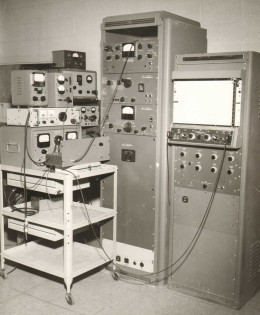
The General Radio model 1390-A
Random Noise Generator is the
upper-most unit on the left side.
The voltage integrator is behind the
unmounted rack panel in the center
(on the cart), and the tall rack enclosure
houses the Technical Products Company
spectrum analyzer.
Photo 5 shows the measurement system (showing a lot of vintage electronic equipment).
6. P-R noise is a good substitute for music when you need a time-stable signal for making a measurement or adjustment. For example, the TDL model 4011 companion to the model 4010 “Restoration Preamplifier” lets you balance the left and right phono cartridge output voltage using a front-panel meter. But the circuit itself needs to be adjusted so that it has same response in both channels. In particular, there is a bandpass filter in each channel which is built using ±1% resistors and ±5% capacitors so there is a small variation between the two passbands. Applying equal pink noise voltages to left and right channel inputs makes this adjustment easy. “Real” music is not sufficiently timestable to do the job.
7. Measuring a loudspeaker’s response is difficult unless you have access to an anechoic chamber (minimal sound reflection but very expensive) or do the testing outdoors with its problems of environmental noise. Reflections from the room is a problem, so a large room with acoustically deadened ceiling, walls, and floor is the next best testing location, but most of us don’t have this option.
But useful testing in a smaller room is possible with some preplanning.
Sound travels at about 1100′ per second with some dependence on temperature and atmospheric pressure, but 1.1′ per millisecond is close enough. You can use a pink noise burst from a “gated” P-R generator if you pay attention to the room size and pulse duration. The setup is shown in Fig. 11. You can use a room as small as 12 × 14′ if the floor is carpeted, the ceiling has acoustical tile, and some sound absorption is used on the walls12. Or, search the Internet for acoustical room treatment or the like.
A noise burst of 10ms should work here, and you can increase this if more sound absorption is added.
A 10 ms burst doesn’t have much energy, so the room needs to be as quiet as possible. Turn off fans and other background noise before making the measurement. Another help is to use the Multi-Instrument software9 and select Linearaveraging and Forever as the averaging time. This lets you accumulate the energy from a series of noise bursts spaced a second or more apart (to allow the room reflections to die out).
In Fig. 11, the speaker to microphone distance is 2-3′ maximum. This “near-field” measurement will accurately show the speaker’s response assuming a microphone and preamplifier with flat frequency responses. A “far-field” measurement always shows the response of the speaker and the room, but this, too, can be useful. Positioning the microphone at your listening position in your listening room can give you insights on adding sound absorption or speaker repositioning. You can use a longer noise burst, 200-300 ms, because you are going to hear the room reflections in your music, so you may as well see them in the noise spectrum. Your goal is to flatten the spectrum, or at least reduce narrow peaks and valleys.
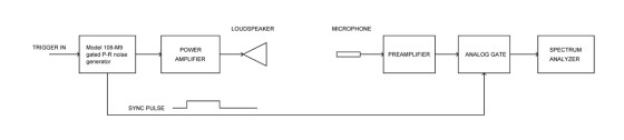
During the 1970s I built noise burst P-R generators (models 108-M5 and 108-M9) for two well-known speaker manufacturers, so I know this method has a history of commercial use. I also built 1/3-octave band spectrum analysis filters for one of the companies, so this is a clue to setting up the spectrum analyzer in Figure 11.
8. Microphone calibration by comparison to a reference microphone can also be done with pink burst noise using the setup shown in Figure 12. Place the reference and un-calibrated mikes side-by-side and in-line with the speaker cone as shown in Photo 6. You can use a noise burst duration of 300 ms because both mikes will “hear” the same reflections. This calibration is best done with the TrueRTA software7 because you can save both the reference mike response and the un-calibrated mike response to the Workbench and then take their difference to get the calibration response.
The speaker’s frequency response does not affect the measurement because both mikes receive the same signal.

is not critical and 15-18″ works fine.

It is important to keep the power input to the speaker and the preamplifier gain constant for both measurements. If the mike sensitivities are different, you can correct this by using the Shift command in the TrueRTA Utilities Menu. Shift the lower curve up until you get the best fit to the upper curve and then take the Difference (also on the Utilities Menu). Third-octave band analysis is a good starting point. Because of the mechanical design of microphones, you should get a smooth difference (calibration) curve.
Final Remarks
Noise can be a useful measurement tool. It is probably under-used because of a lack of understanding, so I hope this article will give you some new measurement ideas. It appears that it may be difficult to find a gated P-R noise generator at this time, so I am designing the TDL model 110. It will produce white and pink noise, have a step and fine output attenuator, and produce noise bursts in 10 ms steps from 10 ms to 490 ms with a sync output.
www.tdl-tech.com
Article originally published in Voice Coil, December 2010
About the author
Ron Tipton has degrees in electrical engineering from New Mexico State University and is retired from an engineering position at White Sands Missile Range. In 1957 he started Testronic Development Laboratory (now TDL Technology, Inc.) to develop audio electronics. During the 1960s and 70s, TDL built active filters and pseudo-random noise generators for well known companies such as Bose Corp. and Acoustic Research. He is still the TDL president and principal designer.
References
1. White noise is defined as having equal energy per unit bandwidth. Pink noise has equal energy per octave bandwidth. Other un-named spectra can be produced with a suitable filter.
2. R.B. Tipton, “A Study of the Stationarity of Laboratory Random Noise Generators,” Proceedings of the IEEE Transactions on Instrumentation and Measurement, March-June 1966.
3. R.P. Gilson, “Some Results of Amplitude Distribution Experiments on Shift Register Generated Pseudo-Random Sequences,” IEEE Transactions on Electronic Computers, December 1966.
4. R.C. White Jr., “Experiments with Digital Computer Simulations of Pseudo-Random Noise Generators,” IEEE Transactions on Electronic Computers, June 1967.
5. Error-Correcting Codes, W.W. Peterson and E.J. Weldon, second edition, 1972, MIT Press.
6. Complete details on the model 109 generator can be found online. Go to www.tdl-tech.com/data109.htm and scroll down to the User Guide.
7. TrueRTA is available from www.trueaudio.com.
8. Audiotester is available from www.audiotester.de. You can download a trial version from their website.
9. Multi-Instrument is available from www.virtins.com. A trial version can be downloaded from their website.
10. Telemetry is “measurement at a distance.” In this article it means using a radio link to send flight performance data from an airborne or space vehicle back to a groundbased station.
11. The year of the Conference and Proceedings was probably 1963. An extensive online search has failed to find this reference so apparently the whole text or even an abstract was not put online. However, the file noisegen.zip on the www.tdl-tech.com/magarts.htm page contains a pdf copy of this paper and Reference.
12. “DIY Room Tune-Up,” Sound and Vision magazine, September 2010, pages 36-39.