When A. N. Thiele and R. H. Small presented their work on loudspeaker modeling in the 1960s and 1970s, it was a revolution for the industry. Instead of guessing a suitable box volume (which could be wrong by as much as a factor of 2) and iterating toward a certain target, simulations could predict the behavior (within reasonable bounds) provided that one knew the Thiele-Small (T-S) parameters beforehand. Loudspeaker technology has evidently progressed significantly since then.
Early 1990s design software included LinearX with its LMS measurement system, and LEAP box and crossover simulations. Today, advanced measurement equipment from Klippel GmbH is standard in laboratories around the world. The older LEAP system is Windows XP-era software and is fading away with no replacement in sight. Interestingly, as transducer manufacturers have become better at measuring their products, and the quality of datasheets have improved, system designers are increasingly leaning on this data and not measuring the drivers prior to designing a system. The data provided are typically simplified T-S parameters, possibly with an indication of the inductance and a few other key parameters.
In spite of the progress, the fundamental quality of loudspeaker parameter estimation and associated box simulation hasn’t changed. It remains based on 1970s T-S parameters and simple mechanical parameters. In reality, the driver exhibits viscoelastic effects in the suspension, and non-inductive elements in the motor that are beyond the physical scope of the T-S model. The difference between the simple T-S model and a more comprehensive model of the driver can potentially be a few decibels when designing a vented system.
Because loudspeakers are no longer designed using pencil-and-paper calculations, more comprehensive new models of the transducer can thus be considered without introducing an impractical amount of calculation for the designer. In particular, we can include viscoelastic damping in the suspension, as well as a voice coil model, including semi-inductive effects. In what follows, we will describe a new advanced model for transducer behavior that we believe is robust enough to serve as a new standard going forward.
Model Parameter Comparison
Table 1 compares the simple parameters (from which the T-S parameters were derived) with our proposed advanced parameter set. Effective cone (shadow) area and force factor (SD and Bl) are common to both models. Whereas the simple model describes the electrical impedance with two parameters, the advanced model uses five. And whereas the simple model describes the motional impedance with three parameters, the advanced model uses four.
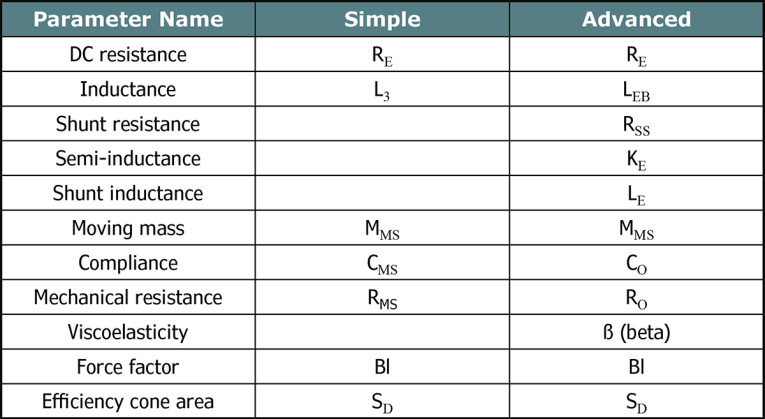
In the simple model, we use a pure inductance (L3), where the subscript denotes matching at the +3dB point. This is an industry convention. The parameter is sometimes named LE and is typically a crude approximation for the true electrical motor impedance. On the mechanical side, a viscoelastic beta parameter has been added in the advanced model. The compliance and mechanical resistance are fundamentally changed and must be recomputed; these are C0, R0. The moving mass MMS retains its usual physical definition.
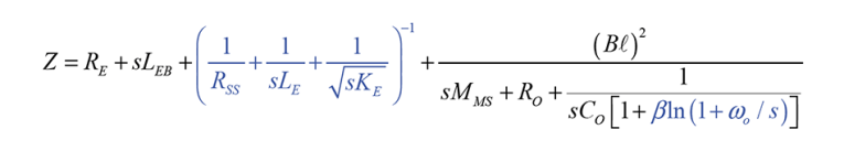
For Equation 1, the black print shows the simple parameters (replace LEB with L3 and R0, C0 with the legacy RMS, CMS) and the blue print shows the additional advanced parameters. We set omega0 to 1.5 times the resonance frequency of the driver. This term provides a cut-off for the viscoelasticity.
Lossless Enclosure: Simple vs. Advanced Models
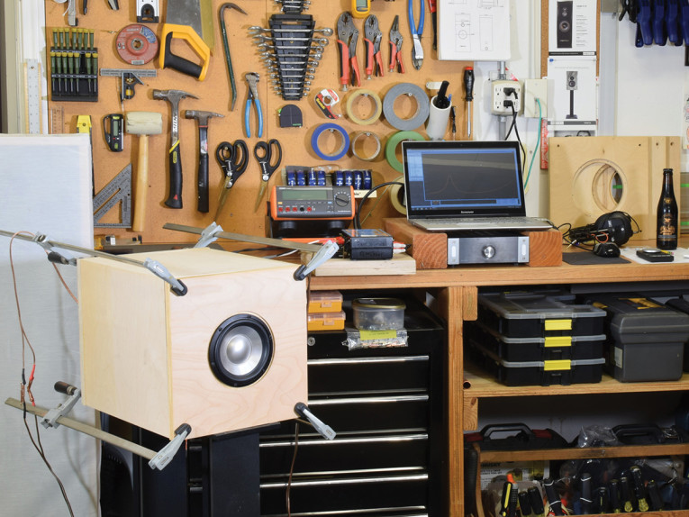
In order to illustrate the magnitude of the correction to be expected when using the advanced model, we present an example based on the SEAS H1488-08 (L16RNX) midwoofer. This midwoofer is simulated in a vented box with volume Vb=26l and port tuning Fp=39.5Hz. All enclosure losses (leakage, port, absorption) are taken to be negligible. Analysis was done using the Speakerbench web application, which we will describe in Part 2 of this article (audioXpress, September 2021). This includes computing the simple and advanced model parameters for the L16RNX, as well as carrying out all box simulations shown in this article.
Note: The 26l box is a readily available box for testing purposes, adaptable to many drivers, and should not be considered a proposal for an optimal box for the L16RNX.
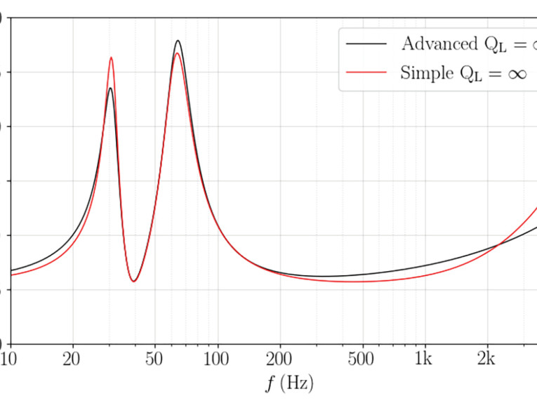
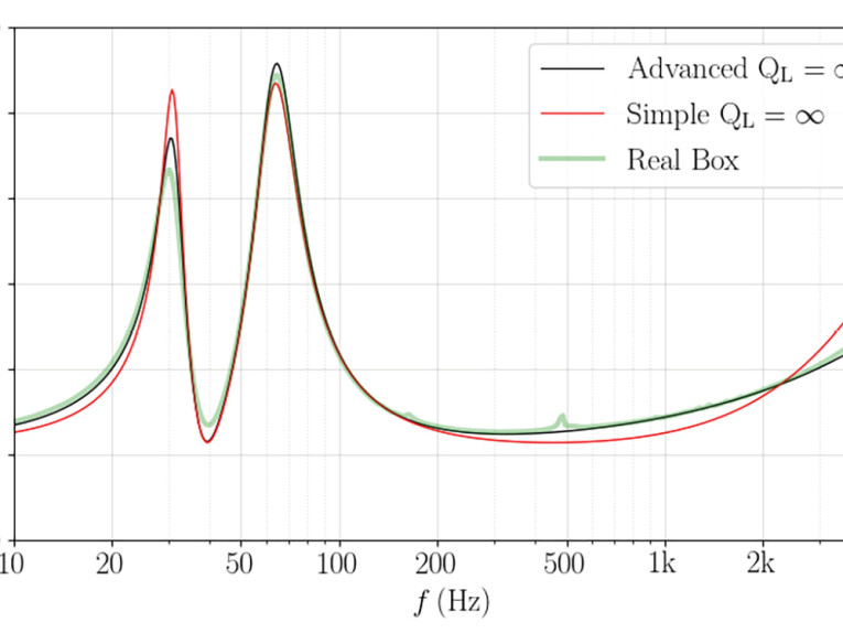
In Figure 1 we plot the total modeled system impedance for the simple (red curve) and advanced (black curve) models. The simple model exhibits the familiar empirical result that both impedance peaks are nearly the same height. In contrast, the advanced model exhibits offset peaks, with the high-frequency (HF) peak increased in amplitude, and the low-frequency (LF) peak reduced in amplitude. This is a manifestation of the frequency-dependent viscoelastic damping.
Lossless Enclosure: Models vs. Reality
Without measurement of the driver in a real enclosure, it is difficult to gauge the absolute accuracy of the simulations. In Figure 2, we measured the midwoofer in a real 26l enclosure, tuned to Fp = 39.5Hz. The measured impedance is shown as the thick green curve. Of course, the real enclosure is not perfectly lossless so we expect the impedance maxima to be reduced in height somewhat in comparison to the lossless simulations.
Note the measured HF peak (green) is above the simple model peak (red). There is no way to correct this result by adding losses to the simple model, as the latter will only reduce the peak height. On the other hand, the advanced model LF and HF peaks (black) are above the measured peaks (green), suggesting that better agreement may be achieved by adding losses to the simulation.
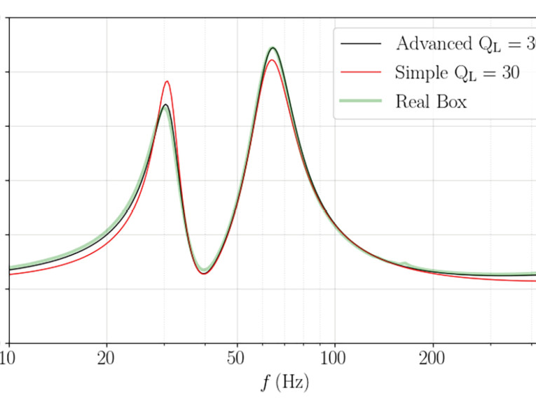
Although there are numerous potential loss channels (leakage, port, absorption), for simplicity we consider only leakage losses. Setting QL = 30 in the simulations give the excellent advanced model result shown in Figure 3. This suggests a total enclosure loss no greater than QB ≈ 30. Importantly, with this loss, the simple model still exhibits the LF/HF overshoot/undershoot of the lossless case, and it is therefore difficult to assess the true magnitude of the enclosure losses with the simple model.
In assessing the losses in practical enclosures, Richard Small (and previous authors) noticed that measured losses exceed theoretical expectations. Small inferred that even though actual leakage loss is insignificant, real enclosure losses present as though QL = 5-10 [1]. For this reason, an engineering rule of thumb emerged such that designers set QL = 7 for modeling purposes.
The analysis presented in the previous sections, however, leads us to suggest that that the anomalous loss (correctly) observed by Small is a result of the driver viscoelasticity that is not included in the simple model. We further claim that corrections (e.g., Small’s rule) are not necessary (and not recommended) when using the advanced model.
Whereas measuring free-field frequency response at low frequencies is practically impossible (requiring a very large anechoic chamber), measuring the impedance of a loudspeaker to very high precision is possible with low-cost equipment. By matching the measured to simulated impedance (as in Figure 3), one can have confidence that the modeled low-frequency SPL is correct (correctly including all losses). Further, potential errors (e.g., a real enclosure leak) is not easily identified in a frequency response measurement, but will be readily apparent in an impedance measurement.
Finally, we remark that Small’s Rule (QL ~ 7) is intended to broadly cover several types of losses (not only leakage but also absorption in the box as well as viscoelasticity of the driver). Box simulations with QL = 7 will cause some error in the frequency response simulation, possibly in the range of 1dB. Ultimately, with the simple model, there is no methodology to arrive at a more correct estimate of losses because the viscoelasticity of the driver is ignored.
Thus Far
In the first part of this article, we have shown that when utilizing an advanced transducer model, very good agreement between box modeling and simulation can be obtained. In Part 2 of this article series, we introduce Speakerbench as our proposal for parameter identification and simple box analysis. aX
This article was originally published in audioXpress, August 2021.
Read part 2 of this article here: Parameter Estimation and Box Simulation with Speakerbench (Part 2) - Introducing Speakerbench
References
[1] R. H. Small, “Vented-Box Loudspeaker Systems — Part 1: Small-Signal Analysis,” Journal of the Engineering Society (JAES), Volume 21, Issue 5, pp. 363-372; June 1973.
About Speakerbench
www.aes.org/e-lib/browse.cfm?elib=1967
 About the Authors
Claus Futtrup received his MSc in ME from Aalborg University in 1997 and has worked in the loudspeaker industry since. From 1997 to 2006, he worked at Dynaudio A/S first as an R&D Engineer, designing loudspeaker boxes and later as a System Engineer for automotive. From 2006 through 2007, Claus was employed as a Transducer Design Engineer at Tymphany in Denmark and in 2008-2013 he was R&D Manager at Scan-Speak. From 2013 to 2015 he worked as Technical Sales Manager for SEAS, Norway, and in 2015 he was promoted to Chief Technical Officer. From August 2021, Claus moved back to Denmark and started working at DALI as manager of the acoustics team.
 Jeff Candy was born in Edmonton, Canada in 1966. He received his Ph.D. in Physics from the University of California, San Diego in 1994, and is currently Director of the Theory and Computational Sciences group at General Atomics in San Diego, CA. He works primarily on theoretical and computational plasma physics, with focus on plasma kinetic theory and turbulence. In the field of audio, he is interested in the application of theoretical acoustics to practical situations. Jeff is a member of the Audio Engineering Society (AES) and a fellow of the American Physical Society (APS). In 2003, he received the Rosenbluth Award for fusion theory, and was 2008 Jubileum Professor at Chalmers University.