From a personal standpoint, I’ve also spent several years using top professional gear (e.g., Audio Precision products) on a daily basis, and that has certainly recalibrated my standards. Of course, pro equipment of that level carries a significant price tag, which is not a big impediment in larger companies, but can be crippling for small labs and individuals who have not won the lottery.
So, all of that said, I thought it would be interesting to see what sort of measurement capability one can achieve using 2021 technology and update my findings and recommendations from the Stone Ages of 2015. Although there’s a lot of options in the low-cost range, I want to demonstrate what a moderate outlay can achieve. So the setup I’m using here, while not cheap, can in many respects outperform the professional gear. I’m very much in the position of a high school violinist who has been practicing on a Stradivarius — the limitations will almost certainly be the user, not the equipment!
Evaluation Hardware
First, a brief mention of the hardware I used in this evaluation. These days, desktop computers are far rarer than 6 years ago, and options for actual sound cards are likewise much more limited. However, external interfaces abound, usually set up as USB devices, and the available performance is astounding. One example is the RME ADI-2 Pro (see Resources), now updated to the FS R model.
The ADI-2 Pro FS R (which I’ll just call ADI-2 for brevity) is capable of a 768kHz sample rate and 24-bit operation. After filtering, the upper frequency limit for the inputs is 180kHz. This is somewhat more restricted than, say, the Audio Precision APx525 that I use for most of my reviews, which samples up to nearly 2.5MHz and has a 1MHz high-frequency limit, but more than generally needed for audio use.
The ADI-2 has balanced inputs that can accept up to 12V signals before overload, and balanced outputs that can output up to 12V. By using the balanced headphone outputs, signals up to 19V can be generated. It also has digital I/O, specifically SPDIF and AES/EBU through coax, XLR, and Toslink.
That said, there’s a lot of other interface choices out there, and the intrepid experimenter can probably find something less expensive that will still offer top performance. I chose the ADI-2 because of its feature set for my uses beyond audio measurement, as well as the raw performance. Oh and also, because it was a generous gift from audioXpress technical editor Jan Didden!
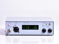
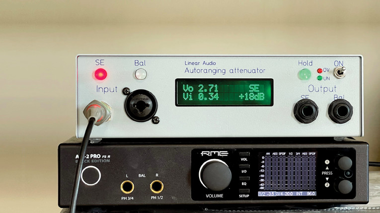
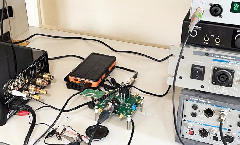
To extend the input voltage range and to speed calibration, I used the Linear Audio Autoranger MkII Measurement Interface (ARII, see Resources). This adds single-ended I/O, voltage gain and attenuation, and calibrated AC voltage measurement to the ADI-2. The combination of these two devices is compact and accessible (Photo 1).
Next, the software, which is really the centerpiece here. Most of the software choices I outlined in my earlier articles are long obsolete. When you see plots from them posted at online forums and blogs, it has that same feel as seeing someone with an AOL or Compuserve email address. But a few have survived and evolved.
For example, Room Equalization Wizard (REW) is an extremely popular freeware package, with a remarkable feature set, constant upgrades, and enthusiastic support from the developer and the users. It’s very easy to use and does a great job with both basic audio measurements (frequency response, distortion) and some fairly sophisticated room and acoustic analysis capabilities. I use it semi-regularly, and manage to slide back into a comfort zone after an hour or so. It’s not quite as intuitive or versatile as the APx software running Audio Precision’s APx-series analyzers, but it’s remarkably good, and the graphics are much more attractive.
ARTA is also still alive, well, and living in my computer. Along with its companion software (STEPS and LIMP), it will handle almost all routine audio measurement (distortion, frequency response, noise, etc.), and is quite intuitive and easy to use. It’s popular and justifiably so.
But if you want something that’s truly professional software in the manner of LabView or MathCAD, Virtins Technologies’ Multi Instrument (MI) offers much broader capability, extending well beyond audio into nearly any kind of electronic instrumentation.
The User Manual is 468 pages of rather terse prose, giving a hint as to the software’s versatility and feature set. I previously wrote about an earlier version of this software, so some of this will necessarily be a bit of a rehash, but the earlier article has a still-valid broad overview.
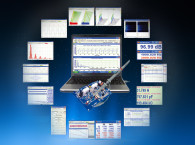
In brief, with the MI package, the user gets an oscilloscope, a signal generator (arbitrary waveform), a spectrum analyzer, a frequency counter, a XY recorder, a signal recorder, an LCR meter, a correlation analyzer, a data logger, a logic analyzer, and more — you get the idea.
The user can select any combination of these instruments to run for an experiment. For example, you can use an oscilloscope, a signal generator, and a spectrum analyzer simultaneously when doing distortion measurements.
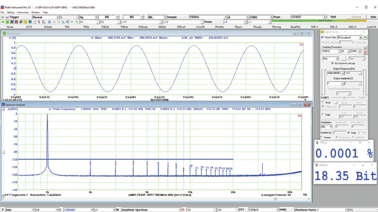
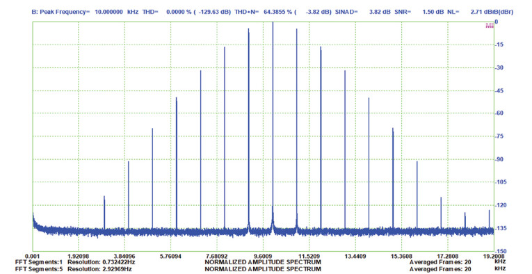
Figure 1 shows a loopback measurement at 1V of the ADI-2 and the ARII, where you can see the automatic measure of THD, THD+N, SINAD, total noise, and signal-to-noise on top of the distortion spectrum.
There are multiple versions and options: I used the fully-equipped MI Pro, and given the relatively low cost of the entire package, I would strongly recommend simplifying your life by shooting for the top. You’ll find that it’s much more than you think you need, but you can grow into the feature set. It’s expensive ($200 to $500) compared to most hobby-level software, but much less expensive than professional measurement software — the price tags of which always contain a comma.
A software key activates the license on a single computer. For a nominal fee, you can get a dongle allowing use on multiple computers (but not simultaneously). Just try not to lose it… You also have several choices of skins, and I still can’t decide if I like white or black backgrounds better, so I’ll be cheerfully inconsistent.
The Instruments (well, some of them)
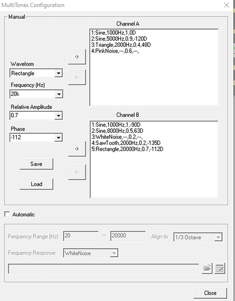
The least superficially impressive looking instrument in the bunch is probably the Signal Generator. But its seemingly simple appearance belies the deep functionality of the virtual instrument. For example, the multitone generator enables the user to pile in any collection of waveforms one could think of, with varying frequencies, wave shapes, and amplitudes. For periodic functions (sine, rectangular, sawtooth, triangle), the relative phase can also be varied, and composite signals can include various noise functions as well.
Figure 2 shows a screenshot of a constructed waveform that I like to call the “Kitchen Sink.” It’s not exactly useful, but it’s a nice encapsulation of the versatility of waveform construction. What can be useful, however, is the ability to add a small amount of white noise to a test signal for dithering. This can allow determination and removal of any quantization distortion in low level measurements.
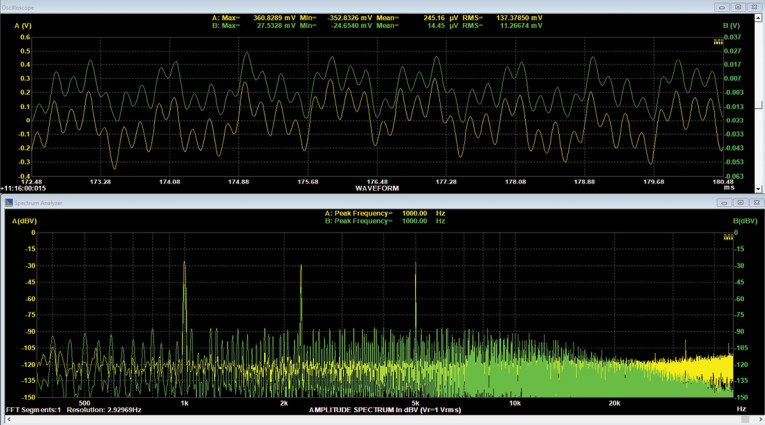
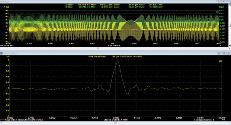
A simpler version was generated with three sine waves of varying frequencies and phases. Figure 3 shows the time and frequency domain of that signal fed into an inexpensive, small amplifier I had on hand. The varying phases can be seen by looking at the envelope of the periodic signal and noting their change from cycle to cycle.
What I didn’t show here, but mentioned in my earlier article, is the innocent-looking “mask” option. The mask (in its simplest form) sets all points within it to zero, so that signal bursts can be generated. The mask can be phase locked to the signal or independent of it. The mask can also be realized as a window function, that is, a defined increase and decrease in amplitude to shape the envelope of the burst.
The signal can also be swept in frequency or amplitude, linear or logarithmic. A nice touch is the ability to have the signal sweep both forward and in reverse. Oh, and did I mention that you can generate FM signals (Figure 4)?
The Spectrum Analyzer is similarly feature-rich. Besides having a ridiculously large number of available windowing functions and being able to do fast Fourier transforms (FFTs) up to 4.2 million points, the spectrum analyzer includes cross-correlation and auto-correlation, as well as measurements like coherence that are derived from the correlation functions.
Figure 5 shows a cross-correlation derived from a frequency sweep (seen in the upper oscilloscope window) between signals measured by the two channels of the ADI-2 in a voltage-current setup described later in this article. The cross-correlation peaks at about 21µs, which is, not coincidentally, one sampling period (fs = 48kHz), neatly measuring the time delay between channels with a complex signal.
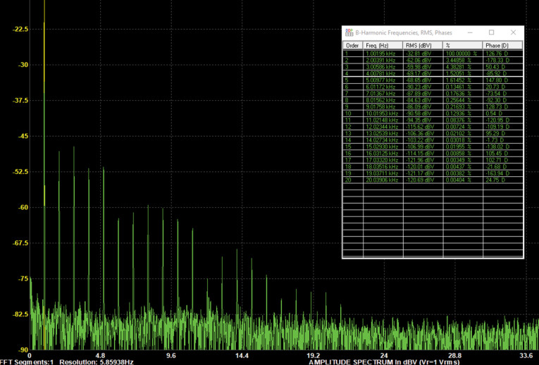
A nice feature of this instrument is the ability to measure not only the magnitude but also the phase of the harmonics. Figure 6 shows the distortion spectrum of an inexpensive lab amplifier along with an MI-generated table of harmonic amplitudes and phases.
As they say on late night TV commercials, “But that’s not all!” MI has a function called Derived Data Points (DDP), which display a numerical value derived from a frame of data; of course, it can be set to update with each acquired data frame. There are more than 200 different options, depending on which instrument is active. You can see examples of the DDPs (in this case, Effective Number of Bits and SINAD) in Figure 1. Further, upper and lower limits on the value can be defined to either set off a visual alarm in the window, sound an alert, or start another process to bring the measured value back into range. For those who want to use MI for statistical process control, the alerts can be set for both control limits and specification limits (in the MI language, “Low-Low, Low, High, High-High”).
MI also enables the user to create User Defined Data Points (UDDP), where the definition contains acquired data, constants, and mathematical functions set up in combination by the user (as the name implies) much in the manner of a spreadsheet. So any sort of customized measurement can be assembled using the building blocks of acquired data. This is an amazingly powerful tool, and as users come up with new needs for measurement metrics, Virtins will often incorporate these needs into the options in succeeding versions.
An example of this is the Total Distortion metric, which using a complex signal as a stimulus, subtracts the scaled input from the output of the device under test (DUT). So if you create a multitoned test signal (e.g., the 42 tone signal I use in many tests) and measure the response to it, MI will report back the total harmonic, intermodulation, and anharmonic components of the measured signal. This addition was in response to a user request on the company’s support forum (see Resources).
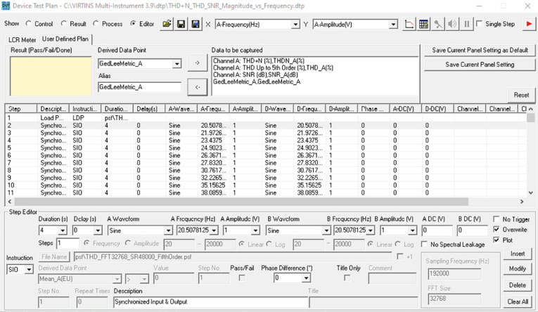
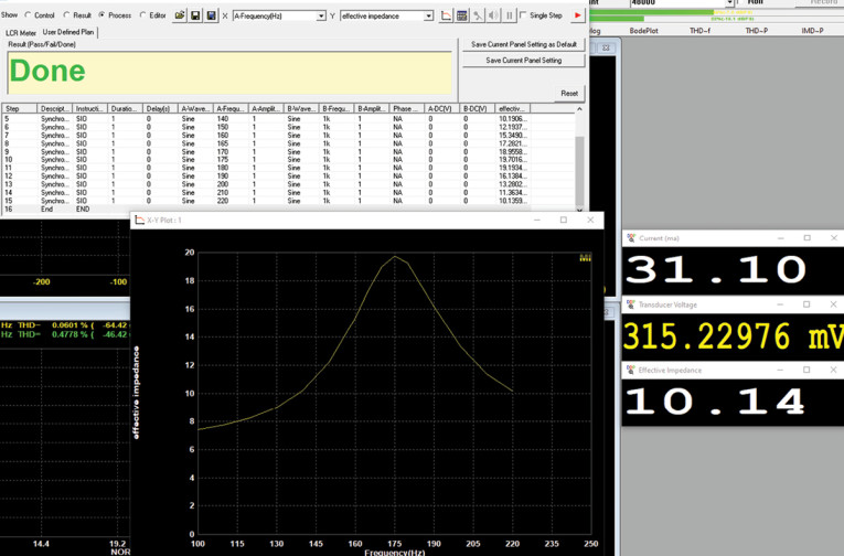
Virtins MI also has a feature called Device Test Plan (DTP), where a sequence of actions (including UDDPs and conditional statements) can be programmed. An example of a DTP being created is shown in Figure 7. The user initiates the Plan and it runs through whatever steps are included. For this specific example, a constant amplitude signal is stepped through varying frequencies to create four charts, THD+N vs. frequency, THD vs. frequency, signal-to-noise vs. frequency, and GedLee Metric vs. frequency. It’s easy to see that the signal amplitude and phase could be varied as well. There are 25 instruction options provided, and up to eight charts can be displayed simultaneously.
A Few Example Measurements
GedLee Metric: For a very long time, audio engineers have been aware that human ears have differing sensitivity to different harmonics, and this varies again with distribution or harmonics and fundamental frequency in a rather complex manner. The upshot is that THD alone is a relatively poor way to characterize the audibility of distortion. Various weighting schemes have been developed over the years to improve the correlation between measured distortion, that is, deviation from a linear transfer function, and perception.
About 20 years ago, the team of Earl Geddes and Lidia Lee developed a rather sophisticated weighting system that took into account the distribution of harmonics, their relative phases (which were not accounted for in earlier weighting schemes), and the overall curvature of the transfer function. This became known as the GedLee Metric (see Resources). The GedLee Metric, Gm, is defined as:

where T(x) is the normalized system transfer function. In this formula, the squared second derivative weights higher-order harmonics more heavily than lower-order harmonics, with squaring used to make any curvature positive independent of direction. The squared cosine term weights deviations near the zero crossing more heavily than at higher values, since cosine is at a maximum at zero and goes to zero at ±π/2, much in the manner of a windowing function.
Geddes and Lee’s data suggested that Gm < 1 would be imperceptible, and 1 < Gm < 3 would be relatively tolerable. There are assumptions in their model of the system being time invariant and non-hysteretic, which is not strictly true for real-world transducers. Nonetheless, the model seems to work well in predicting the audibility of distortion.
To measure the Gm of some speakers I had handy (Vanatoo Transparent 1E powered mini-monitors), I used a PCB Piezotronics 376A32 1/2” condenser lab mic attached to the RME-2’s input via a 48V phantom power supply. The mic was set up about 1 meter from the speaker, and the output level was adjusted to 90dBSPL with pink noise.
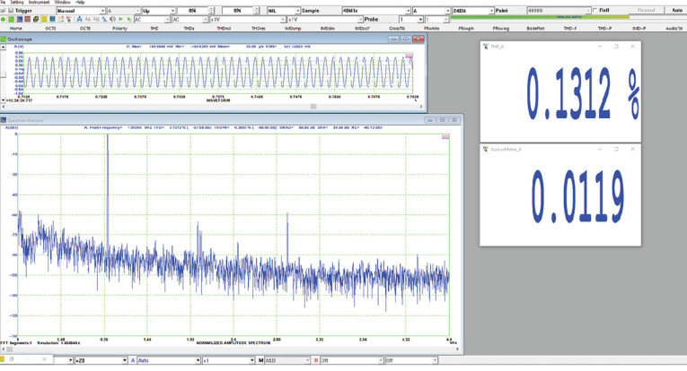
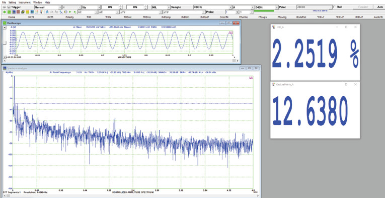
We can get a flavor of what Gm can tell us by comparing it to harmonic distortion measurements at different levels and frequencies. For example, Figure 8 shows the spectrum of a 1kHz sine wave, with a total harmonic distortion (THD) of 0.13%. Subjectively, it sounded quite clean, and the GedLee Metric is indeed well below the detection threshold of 1. Conversely, if we turn the speaker’s limiters off and drive it hard in the bass (31.5Hz), the sound is quite buzzy and unpleasant. Figure 9 shows the THD starting to rise to a bit more than 2%, not a particularly large number at those frequencies. But the GedLee Metric is 12.6, well into the “annoying” range and more accurately describes the perceived level of distortion.
Wow and Flutter
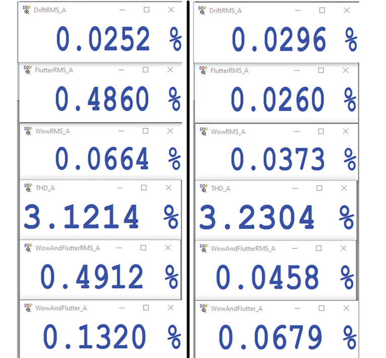
Though the golden days of vinyl are behind us, there’s certainly a strong hobbyist and anachrophile attraction to the medium. Part of the attraction is the technical challenge of extracting high performance from dragging a rock through a piece of plastic. Old timers like me remember the days of wow and flutter (W&F) meters. And in a fit of delicious irony, we can now do W&F measurements using digital technology. Virtins has built this capability into MI with a vengeance—one can measure wow, flutter, wow and flutter, and drift, in both weighted and unweighted modes (see Resources). Figure 10 shows unweighted (left) and weighted (right) measurements for a Technics SP10 Mk3 playing a JIS test tone (3kHz). Of course, you can view frequency and distortion spectra as well. Using the Chart Recorder option, one can even plot the change in frequency over time to determine rotational inconsistencies.
Loudspeaker Drive Measurements
I’ve been playing on and off with some ways to characterize amplifier needs for driving speakers to a desired volume. Most speakers look nothing like a pure resistance, and even as reactances, there’s some “wobble” seen under various drive conditions. I’ve been gathering some data on using real-world signals (music, voices) rather than test tones to characterize this and see, for a given application, what the amplifier will be asked to deliver in terms of both voltage and current at each point in the signal. With the Audio Precision APx1701 transducer interface, this is relatively easy to do, since that box contains the power amplifiers and a series resistance for current sensing.
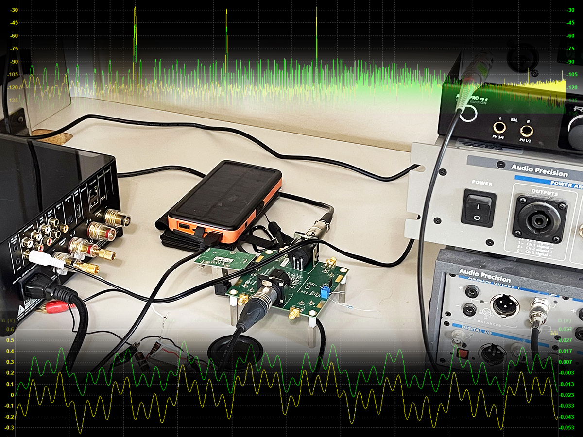
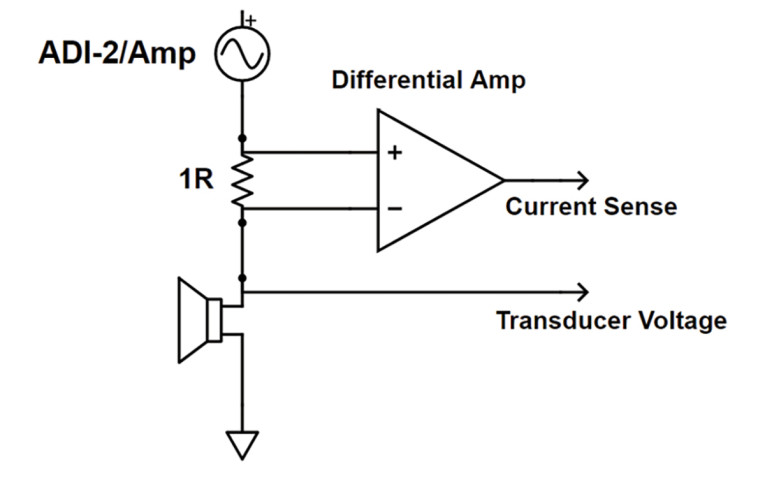
To duplicate this capability, I set up a circuit shown in Figure 11. Voltage across the series sensing resistor is measured using a differential amplifier to remove the main signal across the speaker, which appears as common mode. This can then be converted to current. I chose a 1R resistor to make the math easier (1A = 1V). For a differential amplifier, I used a TI OPA1637EVL board because of the high common mode rejection (CMR) and low noise and distortion. The board was powered via a floating battery and the Linear Audio Silent Switcher power supply. I had some small speaker drivers from Stetron intended for smart speakers, so I used one of them as the test mule. The speaker was driven by an NAD M10 integrated amp, which was overkill, but that amp is small and portable, and I happened to have one nearby. Photo 2 shows the test setup—it is not as elegant as the Audio Precision unit but, putting aside the unnecessarily expensive driving amplifier, it’s much less expensive!
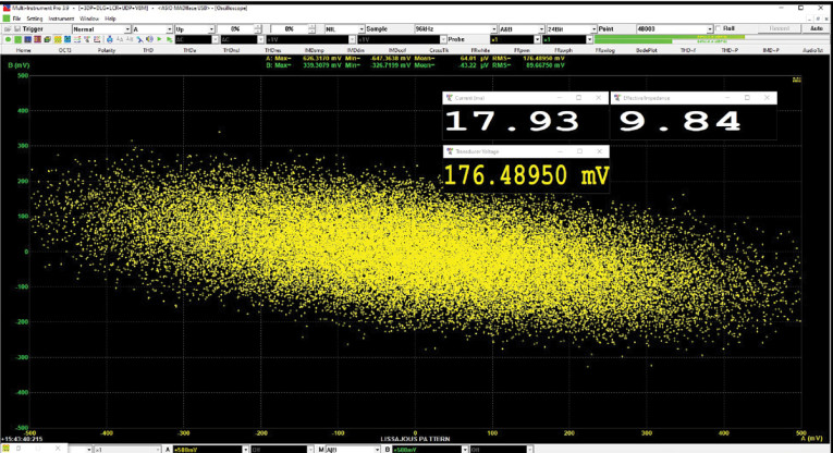
The voltage across the speaker was sent to Channel A, the output voltage of the differential amp (proportional to current) was sent to Channel B. I set up the MI in an X-Y recorder mode (Lissajous) with voltage on the X-axis and current on the Y-axis (1mV = 1mA); you can change the Y-axis label to milliamps (mA) directly if seeing “mV’ bothers you and scale for the sensing resistor size.
Using white noise as a test signal, I got the trace shown in Figure 12, which has a rather galactic look to it. DDPs show the RMS voltage and current, and their ratio, which I termed “effective current.” But still, you can see an area on the I-V plane that an amp is asked to supply, and this can be a useful measure for loudspeakers. Things get even more interesting when using voice and music signals, which I’ll talk about further in coming months.
With MI’s impedance measurement setup, a transducer’s impedance vs. frequency is measured in a two-step process. With a setup like the one shown in Figure 11, the impedance can be measured in one go using a Device Test Plan (Figure 13).
Final Thoughts
Everything technological gets smaller, faster, and less expensive. And measurement gear is no exception. What I have on my bench is about $2,600 worth of equipment and software having noise and distortion capabilities that I could only dream of a few years ago. And that’s being extravagant on the hardware side. I could get 95% of the performance and all of the versatility for half the cost.
As with my last article about the Virtins MI software, I feel that I’ve only scratched the surface with these basic measurement examples. I haven’t mentioned the spectrogram, waterfall, speech intelligibility, cumulative spectral display, digital filtering, and a few dozen more things.
MI admittedly is complex and has a very steep learning curve. It can also do just about anything that you can conceive of for audio test and measurement. While the combination of MI and an interface is far fussier and inconvenient than, say, an Audio Precision analyzer, one can get similar or better results at the expense of efficiency. Whatever it doesn’t do out of the box can be programmed by the user, and as I’ve hinted, you’ll see some interesting uses in my next couple of loudspeaker reviews.
Author Acknowledgements: Besides the kind help and support of the folks at Virtins, I’d like to offer a hat-tip to John Jones and Raoul Jasselette for hints, goads, and generous sharing of data.
Resources
E. Geddes and L. Lee, “Auditory Perception of Nonlinear Distortion—Theory,” 115th Convention of the Audio Engineering Society (AES), October, 2003.
W. Hongwei, “Wow and Flutter Measurement Using Multi-Instrument,”
Virtins Technology,
https://www.virtins.com/doc/Wow-and-Flutter-Measurement-using-Multi-Instrument.pdf
B. Prescott and S. Yaniger, “RME ADI-2 Pro Review,” audioXpress, September 2017,
S. Yaniger, “The Linear Audio Autoranger Mk II Measurement Interface,” audioXpress, April 2020,
S. Yaniger, “The Virtins Multi-Instrument Software,” audioXpress, March 2016,
Virtins User Support Forum, https://www.virtins.com/forum/index.php
This article was originally published in audioXpress, March 2021.
 About the Author
Stuart Yaniger has been designing and building audio equipment for nearly half a century, and currently runs a technology consulting agency in western New York. His professional research interests have spanned theoretical physics, electronics, chemistry, spectroscopy, aerospace, biology, and sensory science. One day, he will figure out what he would like to be when he grows up.