Wavecor’s SW146WA, in both the 8-Ω and 4-Ω versions, have a well-conceived feature set that includes a proprietary four-spoke stamped steel frame that incorporates an eight-spoke/eight-window configuration below the spider mounting shelf. This open eight-spoke region, along with a 13-mm diameter pole vent, provides substantial cooling for the SW146WA. Other features include a stiff flat black coated paper cone, 1.38” (35 mm) diameter convex black coated paper dust cap. Suspension is provided by a low loss (high Qm) nitrile butadiene rubber (NBR) surround plus a 3.25” diameter black flat Conex spider (damper).
All this is driven by a 32-mm diameter (1.25”) voice coil wound with round wire on a black fiber glass nonconducting former. The motor system powering the cone assembly utilizes a single 22-mm × 90-mm ferrite magnet sandwiched between a black plated 4-mm thick front plate and a black plated shaped T-yoke. The SW146WA also uses an aluminum shorting ring (Faraday shield) that reduces distortion caused by eddy currents. Last, the braided voice coil lead wires terminate to a pair of gold terminals.

I began characterizing the new SW146WA using the LinearX LMS analyzer and VIBox to measure both voltage and admittance (current). I generated the sweeps in free air at 0.3, 1, 3, 6, and 10 V. I used the measured Mmd (an actual physical cone assembly measurement with 50% of the surround and spider removed) provided by Wavecor rather than a single 1-V added (delta) mass measurement.
It should also be noted that this multi-voltage parameter test procedure includes heating the voice coil between sweeps for progressively longer periods to simulate operating temperatures at that voltage level (raising the temperature to the first and second time constants).
I further processed the 12 sine wave sweeps for each woofer and divided the voltage curves by the current curves to produce impedance curves. I used the LEAP phase calculation routine to generate the phase curves, after which I copy/pasted the impedance magnitude, phase curves, and associated voltage curves into the LEAP 5 Enclosure Shop software’s Guide Curve library. Then, I used this data to calculate the parameters, using the LEAP 5 LTD transducer model. Because most manufacturing data is produced using a standard transducer model or in many cases the LEAP 4 TSL model, I also generated LEAP 4 TSL model parameters using the 1-V free air, which can also be compared with the manufacturer’s data.
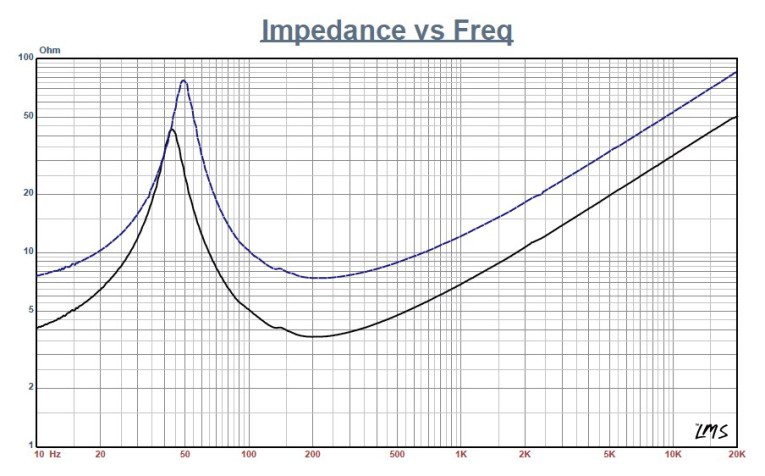
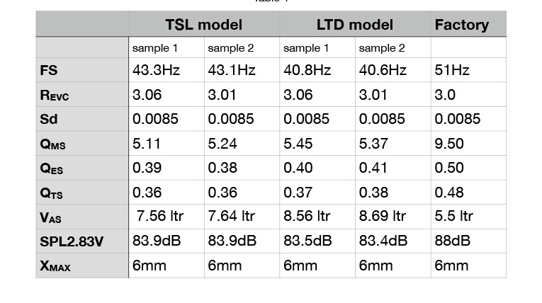
Figure 1 shows the SW146WA01/02’s 1-V free-air impedance plots. Table 1 compares the LEAP 5 LTD and LEAP 4 TSL Thiele-Small (T-S) parameter sets for the Wavecor SW146WA01 driver samples along with the Wavecor factory data. Table 2 shows the same data for the 8-Ω SW146WA02 version.

The SW146WA01’s comparative data shows that all four parameter sets for the two samples were reasonably similar and correlated well with the factory data with very close Fs/Qt ratios. The biggest discrepancy was the sensitivity. The SW146WA02 had even better correlation with the factory data and much closer sensitivity prediction.
Following Test Bench protocol, I used the Sample 1 LEAP 5 LTD parameters for each version and set up two computer box simulations, both in the same 0.35-ft3 Chebychev/Butterworth-type vented alignment, tuned to 38 Hz with 15% fill material (fiberglass). I performed the first simulation using the SW146WA02 8-Ω version, and the second using the SW146WA01 4-Ω version. While I did this alignment with a simulated port tube, this low of a tuning in this small of an enclosure would be well suited to using a passive radiator.
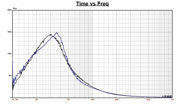
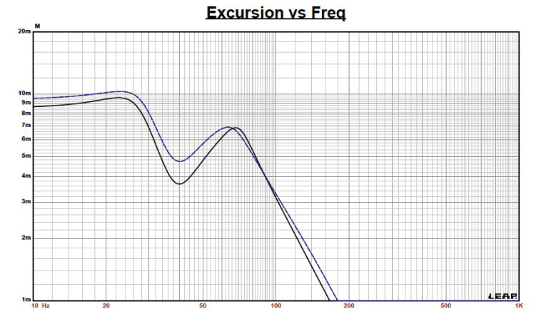
Figure 2 shows the results for the Wavecor SW146WA01/02 in the vented enclosures at 2.83 V and at a voltage level sufficiently high enough to increase cone excursion to 6.9 mm (XMAX + 15%). This resulted in a F3 of 51.7 Hz (–6 dB = 39.5 Hz) for the 8-Ω vented simulation; and with the 4-Ω version in the same enclosure, F3 = 46.8 Hz (F6 = 37 Hz). Increasing the voltage input to the simulations until the approximate XMAX + 15% maximum linear cone excursion point was reached resulted in 103.58 dB at 22.5 V for the 8-Ω vented enclosure simulation and 103 dB with a 16-V input level for the 4-Ω vented box. Figure 3 and Figure 4 show the 2.83-V group delay curves and the 22.5-V/16-V excursion curves, respectively.


Klippel analysis for the SW146WA01 4-Ω version produced the data shown in Figures 5–8 (the 8 Ω was not done separately, as the data would be very similar). Our analyzer is provided courtesy of Klippel GmbH. Patrick Turnmire, of Redrock Acoustics, performed the tests. Please note, if you do not own a Klippel analyzer and would like to generate this type of data on any transducer, Redrock Acoustics can provide Klippel analysis. For more information, visit www.redrockacoustics.com.
The SW2146WA01’s Bl(X) curve shown in Figure 5 is nicely broad, especially for this diameter driver, and symmetrical, which is typical of a driver with a relatively high XMAX. The Bl symmetry curve shown in Figure 6 shows a small and not significant 0.9-mm Bl coil-out (forward) offset at rest, which transitions to less than 0.1-mm offset from 4 mm to its maximum excursion.
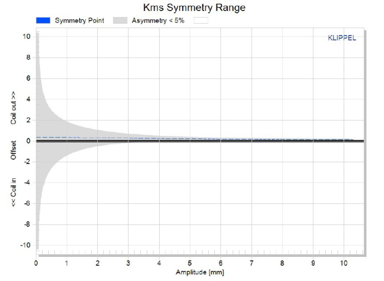
Figure 7 and Figure 8 show the KMS(X) and KMS symmetry curves. Like the Bl curve, the KMS stiffness of compliance curve is very symmetrical, with only a minor offset (see Figure 7). The KMS symmetry range curve exhibits a minor 0.4 mm coil-out offset at rest that decreases to 0.19 mm at the physical XMAX.
Displacement limiting numbers calculated by the Klippel analyzer for the SW146WA01, using the subwoofer criteria for Bl, was XBl at 70% (Bl dropping to 70% of its maximum value) equal to 6.9 mm for the prescribed 20% distortion level (the criterion for subwoofers). For the compliance, crossover at 50% CMS minimum was 7.5 mm, which means that for this Wavecor subwoofer, the Bl is the more limiting factor for getting to the 20% distortion level. however, this number is greater than the physical XMAX of the SW146WA. This is excellent performance.
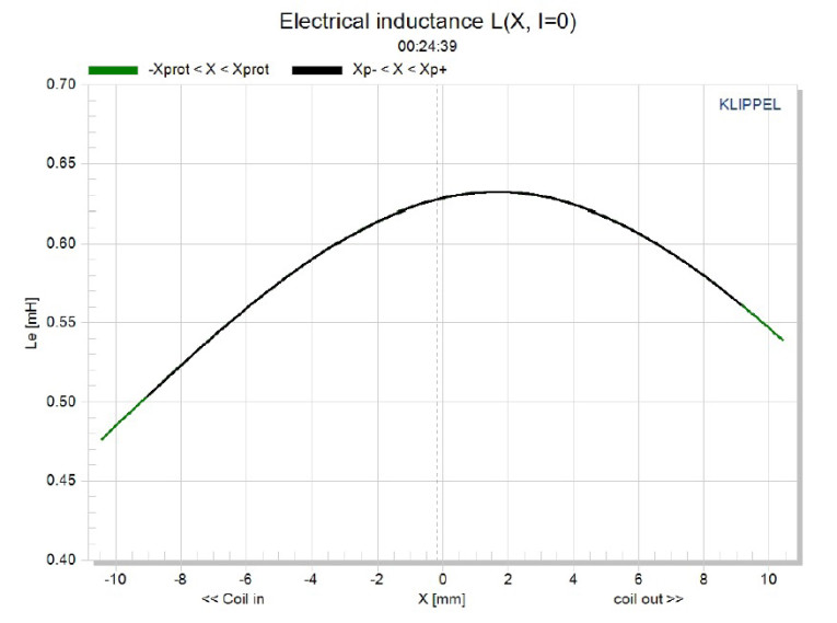
Figure 9 shows the inductance curve Le(X). Motor inductance will typically increase in the rear direction from the zero rest position and decrease in the forward direction as the voice coil moves out of the gap and has less pole coverage. However, that doesn’t happen here. What we do get is lower inductance variation from full in to full out travel, which is the goal. It’s easy to see the benefit of the aluminum shorting ring with inductance only varying from 0.07 to 0.3 mH, which is very good indeed.
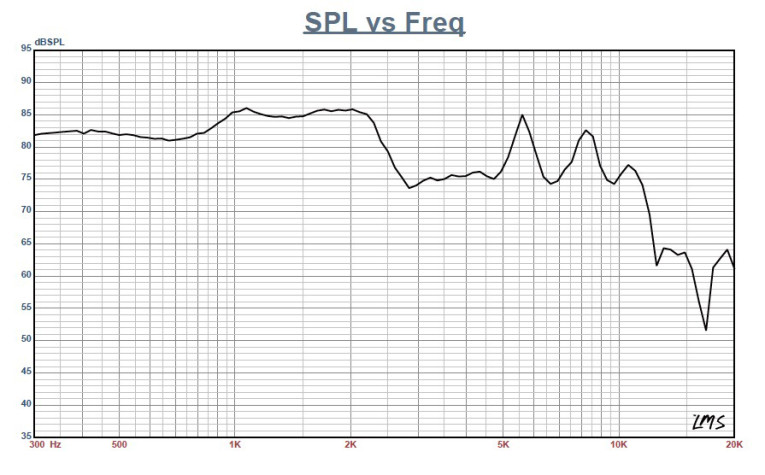
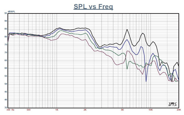
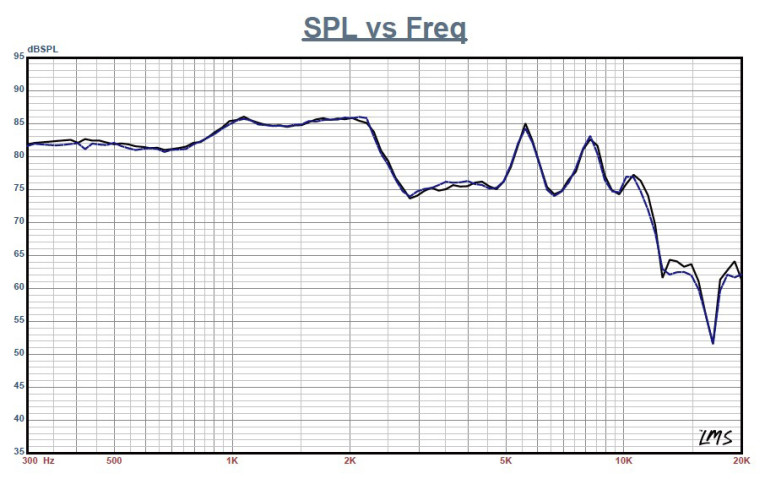
Next, I mounted the driver in a large enclosure filled with foam damping material and that had a 12” × 7” baffle area. I used the LMS gated sine wave technique to measure the SW146WA01/02’s sound pressure level (SPL) on-axis (for both the 4-Ω and the 8-Ω versions) and off-axis (using only the 4-Ω version). Figure 10 shows the on-axis response measured from 300 Hz to 20 kHz at 2.83 V/1 m. The response is a smooth ±3 dB out to 2 kHz for both impedance versions of this driver. Figure 11 shows the SW146WA01’s on and off axis from 0° to 45°. Even though this is a subwoofer, it certainly would be possible to use it in a two-way configuration with a low-pass crossover frequency at high as 1–2 kHz to a tweeter or a large planar transducer.
Finally, Figure 12 shows the SW146WA01’s two-sample SPL comparison showing the drivers to be well matched. Next, I used the Listen SoundCheck analyzer to perform distortion and time-domain analysis on the SW146WA01 (since I would expect similar results for both versions, I did not produce this data for the SW146WA02). For the distortion measurements, I rigidly mounted the driver in free air and increased the voltage until it produced a 1 m SPL of 94 dB (8 V). Note that 94 dB is my SPL standard for measuring distortion in home audio drivers.
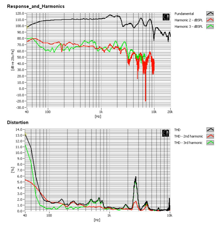

Then, I measured the distortion with the microphone placed near-field about 10 cm from the dust cap (see Figure 13), which actually includes two plots—the top graph is the standard fundamental SPL curve with the second and third harmonic curves, and the bottom graph is the second and third harmonic curves plus the total harmonic distortion (THD) curve with an appropriate X-axis scale. Interpreting the subjective value of conventional distortion curves is almost impossible. However, looking at the relationship of the second to third-harmonic distortion curves is of value.
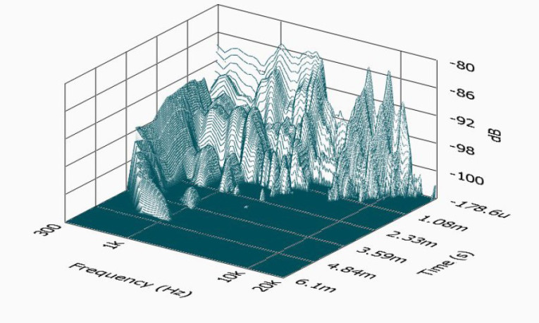
I then used SoundCheck to get a 2.83 V/1 m impulse response (again with the driver mounted in the enclosure with the 15” × 9” baffle) and imported the data into Listen’s SoundMap Time/Frequency software. Figure 14 shows the resulting cumulative spectral decay (CSD) waterfall plot. Figure 15 shows the Wigner-Ville (for its better low-frequency performance) plot. The SW146WA01/02 is another well-crafted transducer from the engineers at Wavecor.
www.wavecor.com
This article was originally published in Voice Coil, July 2015.