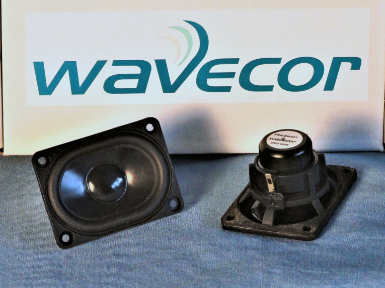
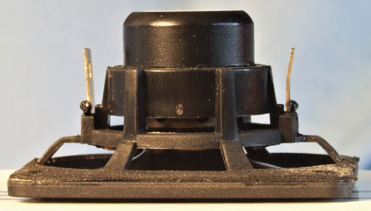
This new Wavecor full range, the FR4X6WA01, is a 4cm × 6cm oval diaphragm driver that can be seen in Photo 1. This device is built on a proprietary injection molded polymer four-spoke frame. Like most contemporary drivers, the area below the spider mounting shelf is totally open for increased cooling (Photo 2). The racetrack 1.75” × 2.5” cone assembly consists of a black anodized aluminum cone with a 16mm diameter round black anodized aluminum dust cap. The black aluminum dust cap is directly coupled to the 16mm vented black non-conducting black fiberglass voice coil former, and suspended with a low loss (high Qm) NBR rubber surround and a 33mm diameter flat Conex spider (damper). Powering the cone assembly is a dual neodymium motor with a copper cap shorting ring (Faraday shield) and a milled return cup with black emissive coating. Tinsel leads connect on one side of the cone to a pair of solderable gold-plated terminals located on opposite sides of the frame, which discourages rocking modes.
I began testing the Wavecor FR4X6WA01 using the LinearX LMS analyzer and the Physical Lab IMP Box. Please note that the Physical Lab (www.physical-lab.com) IMP Box measures current and voltage measurements exactly the same as the LinearX VIBox, however, the LinearX VIBox is no longer available. This was used to create both voltage and admittance (current) curves with the driver clamped to a rigid test fixture in free-air at 0.3V, 1V, 3V, and 6V. However, the 6V curves were not linear enough for LEAP 5 to get a good curve fit, which is typical for this small a diameter driver.
As has become the protocol for Test Bench testing, I no longer use a single added mass measurement and instead used actual measured mass, the manufacturer’s measured Mmd data (1.37 grams). Next, I post-processed the six 550-point stepped sine wave sweeps for each of the FR4X6WA01samples and divided the voltage curves by the current curves (admittance) to produce the impedance curves, phase generated by the LMS calculation method. I imported the data, along with the accompanying voltage curves, to the LEAP 5 Enclosure Shop software.
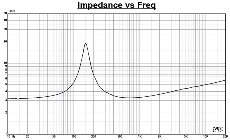
Since most Thiele-Small (T-S) data provided by OEM manufacturers is produced using either a standard driver model or the LEAP 4 TSL model, I additionally created a LEAP 4 TSL model using the 1V free-air curves. I selected the complete data set, the multiple voltage impedance curves for the LTD model, and the 1V impedance curve for the TSL model in the transducer derivation menu in LEAP 5 and created the parameters for the computer box simulations. Figure 1 shows the 1V free-air impedance curve. Table 1 compares the LEAP 5 LTD and TSL data and factory parameters for both of the FR4X6WA01 samples.

LEAP TSL/LTD parameter calculation results were reasonably close to the factory data, with Fs/Qt ratios being in the same “ballpark.” Following my usual protocol, I configured computer enclosure simulations using the LEAP LTD parameters for Sample 1. This consisted of a 15in3 Chebychev sealed box with 50% damping material (fiberglass), and a 51in3 Chebychev/Butterworth vented enclosure tuned to 88Hz with 15% damping material in the box.
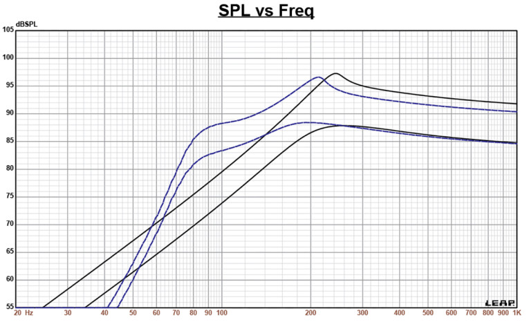
Figure 2 displays the results for the Wavecor driver in the sealed and vented box simulations at 2.83V and at a voltage level sufficiently high enough to increase cone excursion to Xmax+15% (2.3mm for the FR4X6). This produced a F3 frequency of 178Hz (F6=150Hz) with a Qtc=1.16 for the 15in3 Chebychev sealed enclosure and –3dB=129Hz (F6=87Hz) for the 51in3 Chebychev/ Butterworth vented simulation. Increasing the voltage input to the simulations until the maximum linear cone excursion was reached resulted in 97.2dB at 7.3V for the sealed enclosure simulation and 96.5dB for the 6V input level for the Chebychev/Butterworth vented enclosure. Figure 3 shows the 2.83V group delay curves. Figure 4 shows the 7.3V/6V excursion curves.

Klippel analysis for the Wavecor FR4X6WA01 oval full-range driver was provided this month by Warkwyn (Jason Cochrane performed the analysis) with the Klippel KA3 analyzer produced the Bl(X), Kms(X) and Bl and Kms symmetry range plots given in Figures 5-8. The Bl(X) curve for the FR4X6WA01 (Figure 5) is fairly narrow, but is rather symmetrical with fairly minor amount of offset to the curve, but not bad for a short Xmax 15cm2 Sd driver. Looking at the Bl symmetry plot (Figure 6), this curve shows a minor coil-out (forward) offset that remains mostly constant at 0.25mm out to the physical 2mm Xmax of the driver.


Figure 7 and Figure 8 show the Kms(X) and Kms symmetry range curves for the Wavecor full-range driver. The Kms(X) (Figure 7) curve is also rather symmetrical, with a small amount of forward offset. Looking at the KMS symmetry range curve shown in Figure 8, there is about 0.38mm forward offset at 1mm deceasing to 0.27mm at the 2mm physical Xmax position, which is negligible. Displacement limiting numbers calculated by the Klippel analyzer for the Wavecor full-range driver were XBl @ 82% Bl is 1.6mm and for XC at 75% Cms minimum was 1.4mm, which means that for this woofer compliance is the most limiting factor for prescribed distortion level of 10%. Using the more conservative XBl@70% and XC@50%, the criteria for 20% distortion level, XBl=2.12 and XC=2.29, both greater than the 2mm physical Xmax of the driver. Given the small excursion difference between the two distortion criteria, this is very good performance for a small oval
1.5” × 2.5” device.
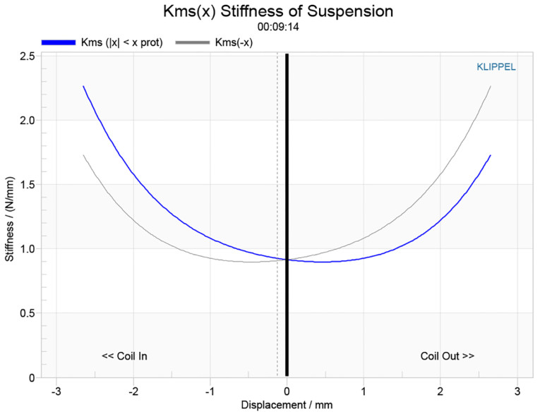
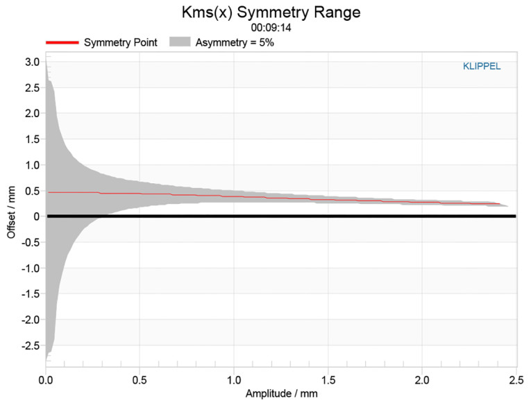
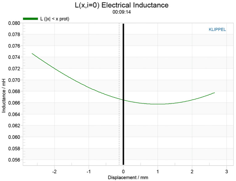
Figure 9 gives the inductance curve Le(X) for the FR4X6WA01. Inductance will typically increase in the rear direction from the zero rest position as the voice coil covers more pole area. However, this device has a copper shorting ring, so the inductance variation is only a maximum of 0.006mH from the in and out Xmax positions, which is very good indeed.
Next, I mounted the FR4X6WA01 full-range driver in an enclosure, which had a 9” × 4” baffle and was filled with damping material (foam). Then, I measured the transducer on- and off-axis from 300Hz to 40kHz frequency response using the Loudsoft FINE R+D analyzer and the GRAS 46BE microphone (courtesy of Loudsoft and GRAS Sound & Vibration) both on and off-axis from at 2.0V/0.5m, normalized to 2.83V/1m using the cosine windowed FFT method. All of these SPL measurements also included a 1/6 octave smoothing, which approximate the 100-point frequency response resolution I used with LMS for a number of years.
Figure 10 gives the FR4X6WA01 on-axis frequency response, which exhibits a smooth rising from 200Hz to above 20kHz. The response extends out to about 40kHz, without really significant aluminum break-up modes. This rising response will be baffle dependent, but a small amount of contour filtering will render it more flat. Figure 11 displays the on- and off-axis frequency response at 0°, 15°, 30°, and 45°.

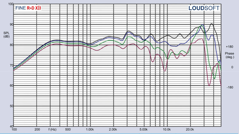
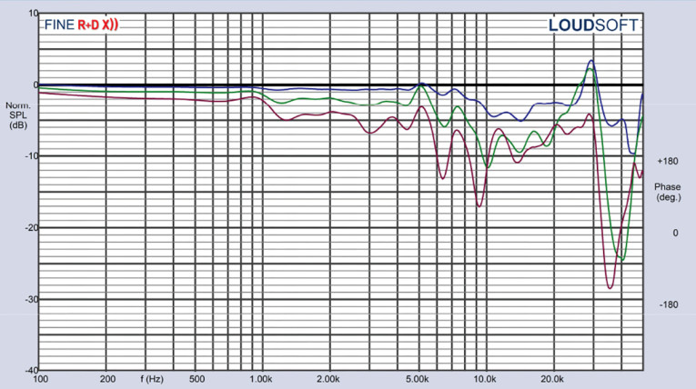
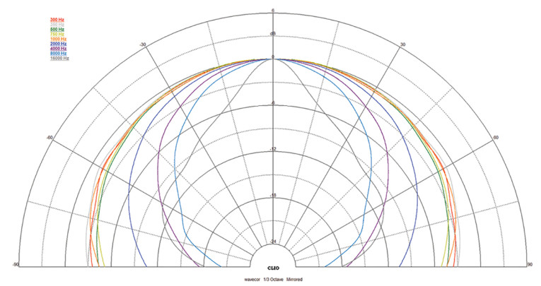
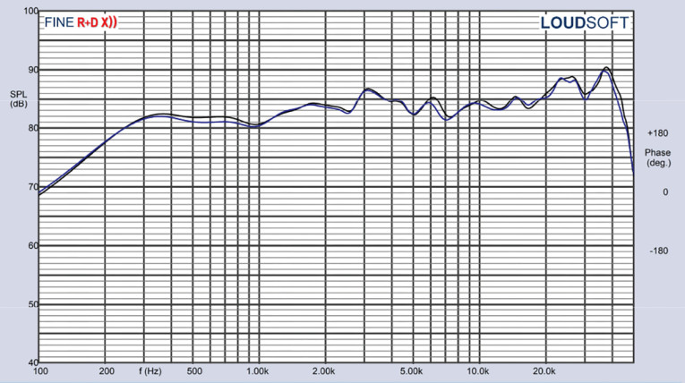
Figure 12 gives the Figure 11 off-axis curves normalized to the on-axis response. Figure 13 shows the CLIO 180° polar plot (measured in 10° increments). Figure 14 shows the two-sample SPL comparison, indicating the two samples were closely matched within less than 1.5dB out to 40kHz. In addition to these normal SPL tests, I also wanted to ascertain if the oval shape produced any directivity issues. I compared the 30° off-axis SPL with the FR4X6WA01 mounted both horizontally and vertically, as shown in Figure 15. As can be seen, the impact is pretty minimal up to 10kHz, so I don’t think directivity issues should be a primary concern when determining a mounting axis.

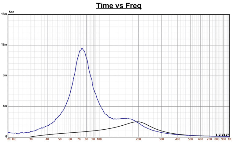
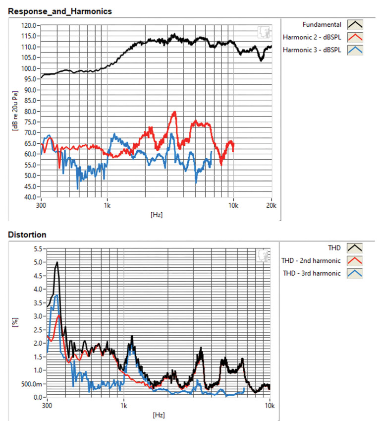
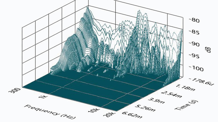
For the remaining series of tests, I employed the Listen SoundCheck 20 software, along with the AudioConnect analyzer with the Listen ¼” SCM microphone and power supply (courtesy of Listen, Inc.) to measure distortion and generate time-frequency plots. For the distortion measurement, the Wavecor 1.75” × 2.5” oval full-range driver was mounted rigidly in free-air, and the SPL set to 90dB at 1m (6.0V), using a noise stimulus. Then, I measured the distortion with the microphone placed 10cm from the dust cap. This produced the distortion curves shown in Figure 16. I then used SoundCheck to get a 2.83V/1m impulse response for this driver and imported the data into Listen’s SoundMap Time/Frequency software. Figure 17 shows the resulting CSD waterfall plot. Figure 18 shows the Short Time Fourier Transform (STFT) plot.

Looking over all the above data, the new Wavecor driver should find application in any number of projects from Bluetooth speakers to computer monitors, or possibly in pro sound line arrays. With all the features Wavecor has incorporated into this microspeaker category device, such as copper shorting rings, vented cone, non-conducting voice coil former, and black emissive coatings on the motor assembly, this is actually a fairly high-end transducer when compared to the many of the drivers in the category. For more information, visit www.wavecor.com. VC
This article was originally published in Voice Coil, November 2022