In 2016, Oxeon successfully applied its TeXtreme thin-ply carbon reinforcements to create a new type of speaker diaphragm. The significant technical and commercial success led Oxeon to spin off its audio related business to a dedicated, highly focused company — Composite Sound. The correct terminology for these cones is Thin-ply Carbon Diaphragms (TPCD). For more information, the Industry Watch section of the February 2022 issue of Voice Coil has a great article about TPCD cones written by Composite Sound’s Martin Turesson, (available online here).
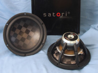
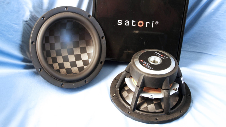
For this Test Bench, SB Acoustics sent its new 9.5” Satori WO24TX-4 TPCD cone woofer (Photo 1). As such, the SB Acoustic WO24TX-4 TPCD cone 9.5” woofer is the fifth TPCD diaphragm transducer to be explicated in Test Bench. The first one was the Eminence N314X-8 compression driver (May 2020), followed by the SB Acoustics TW29TXN-B-4 tweeter (September 2020), the SB MW16TX-4 woofer (June 2021), the SB MW13TX-4 woofer (January 2022), and the SB MW19TX-8 woofer (February 2022). TPCD diaphragms are finding acceptance among loudspeaker manufacturers over the last several years. While SB Acoustics was one of the first OEMs to start using TPCD cones, SEAS has recently announced a new line of transducers based on TPCD.
In the studio monitor market, Ex Machina Soundworks uses a TPCD midrange cone in a coax driver (based on the SEAS King Coax) for both of their monitors priced at $8000 to $11,500, plus THX-certified the Perlisten Audio’s $15,000/pair S7t tower, which uses four 6.5” TPCD market, it’s obvious that this relatively new diaphragm material has gained a fair amount of attention and acceptance rather quickly, somewhat like Beryllium did a few years back.
The SB Acoustics WO24TX-4 is from the SB Satori line of high-end transducers and has a substantial feature set that begins with a proprietary six-spoke cast-aluminum frame, comprised of fairly narrow (about 18mm×17mm) spokes, completely open below the spider (damper) mounting shelf for cooling. Additional cooling for this driver is provided by a 21mm diameter pole vent with a flared exit.
The cone assembly consists of a curvilinear inverted single piece “bowl” shaped cone. The cone is glued to a conventional-looking conic section of TPCD joining the cone to a normal-looking voice coil next joint. Compliance is provided by NBR surround that has a shallow transition to the cone attachment, with the remaining compliance coming from a 4.25” diameter flat spider (damper). This spider is a series of eight 10mm diameter holds punched around its peripheral.
The motor is a FEA-optimized neodymium magnet-type with milled plates and an undercut pole piece with dual copper shorting rings (Faraday shield). Driving the cone assembly is a 49.5mm (1.95”) diameter voice coil wound with round copper-clad aluminum wire (CCAW) on a non-conducting vented fiberglass former. Last, the IEC 268-5 power handling is rated at 90W and the voice coil silver lead wires are terminated to gold-plated solderable terminals located on opposite sides of the former to discourage rocking modes.
I began testing the woofer using the LinearX LMS analyzer and the Physical LAB IMP Box (the same type fixture as a LinearX VI Box) to create both voltage and admittance (current) curves with the driver clamped to a rigid test fixture in free-air at 0.3V, 1V, 3V, 6V, 10V, 15V, and 20V with the oscillator turned on at 200Hz between sweeps to simulate the actual temperature increase over time to reach the third time constant. The 20V curves were too nonlinear to get a sufficient curve fit and were discarded.
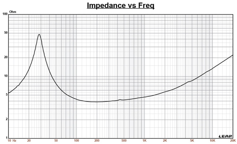
Following my established protocol for Test Bench testing, I no longer use a single added mass measurement. Instead I use the physically measured Mmd data (40.5 grams for the WO24TX-4). The measured data, in this case the 12 550-point (0.3V to 15V) sine wave sweeps for each SB Acoustics sample were post-processed and the voltage curves divided by the current curves to generate impedance curves, with the phase derived using the LMS calculation method. That data, along with the accompanying voltage curves, was imported to the LEAP 5 Enclosure Shop software. Figure 1 shows the 1V free-air impedance curve. The 1V TSL data was selected in the transducer parameter derivation menu in LEAP 5 and the parameters created for the computer box simulations. Table 1 compares the LEAP 5 LTD/TSL Thiele-Small parameter data and factory parameters for both of SB WO24TX-4 samples.
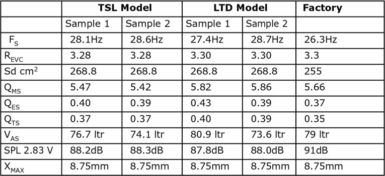
LEAP LTD and TSL parameter calculation results correlated well with the SB Acoustics published data. As I normally do in this column, I followed my established protocol and proceeded to set up computer enclosure simulations using the LEAP LTD parameters for Sample 1. Two simulated enclosures were programmed into the LEAP 5 software — one Butterworth Qtc=0.7 sealed box with 1ft3 air volume with 50% damping material (fiberglass) and a vented Quasi Third-Order Butterworth (QB3) alignment with a 1.8ft3 volume with 15% damping material tuned to 28Hz.
Figure 2 displays the enclosure simulation results for the WO24TX-4 woofer in the sealed and vented enclosures at 2.83V and at a voltage level that achieves excursion equal to Xmax+15% (10.1mm for the WO24TX-4). This resulted in a F3 of 48Hz (-6dB=38Hz) with a Qtc=0.7 for the closed box and a -3dB for the vented simulation of 36Hz (-6dB=29Hz). Increasing the voltage input to the simulations until the Xmax+15% excursion was reached resulted in 111.2dB at 30V for the sealed enclosure simulation and 112.1dB with the same 30V input level for the larger vented box.
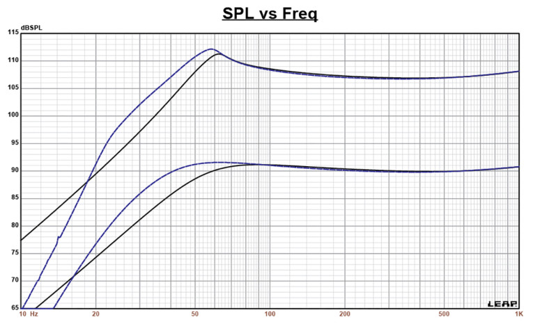
Figure 3 shows the 2.83V group delay curves. Figure 4 shows the 30V excursion curves. While the excursion of the WO24TX-4 doesn’t increase radically below the tuning frequency, like all vented box woofers, it would benefit from a steep high-pass filter below the tuning frequency. Klippel analysis for the SB Acoustics 9.5” woofer was performed by Warkwyn’s Jason Cochrane, using the Klippel KA3 analyzer. The Bl(X) curve for WO24TX-4 (Figure 5) is fairly broad like any high Xmax driver, but with a very small degree of “tilt” coil-in to coil-in and is rather symmetrical. The Bl symmetry curve (Figure 6) shows a small 0.4mm Bl coil-in (rearward) offset once you reach an area of reasonable certainty (about 6mm) and progressively decreasing to a negligible 0.11mm coil-out offset at the 8.75mm physical Xmax excursion point.
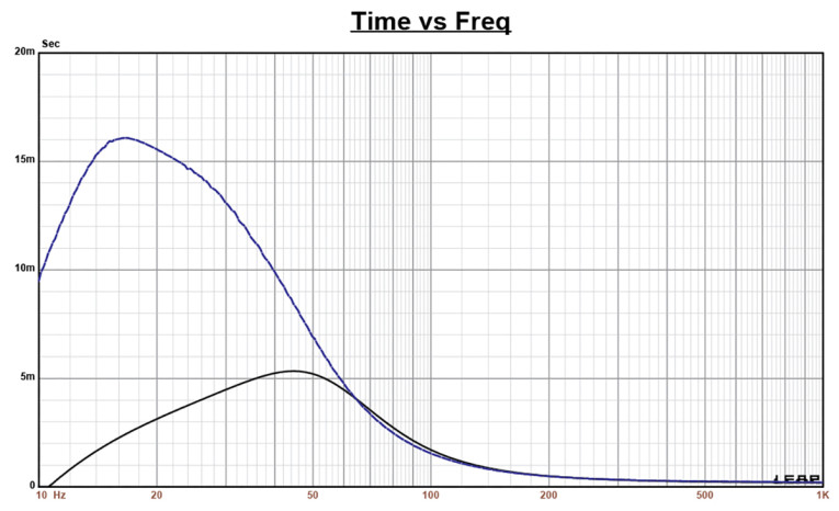
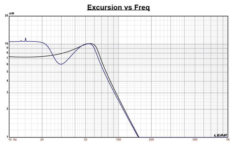
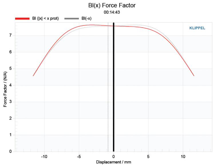
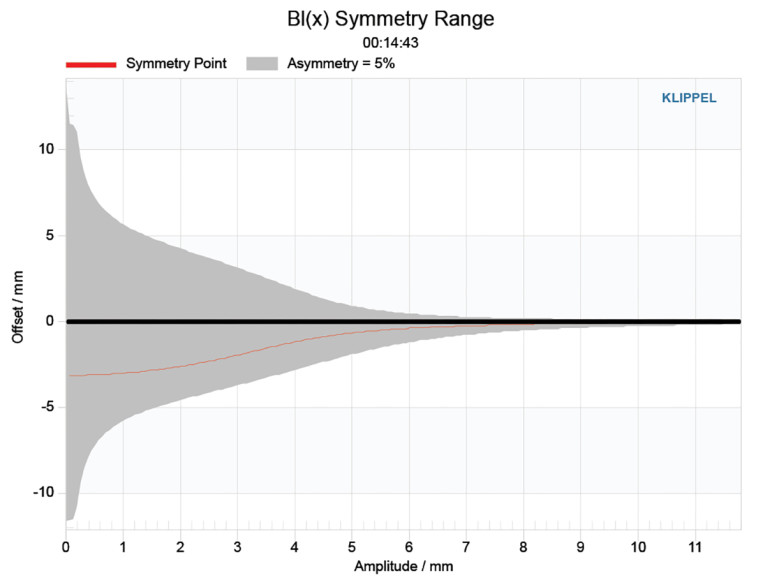
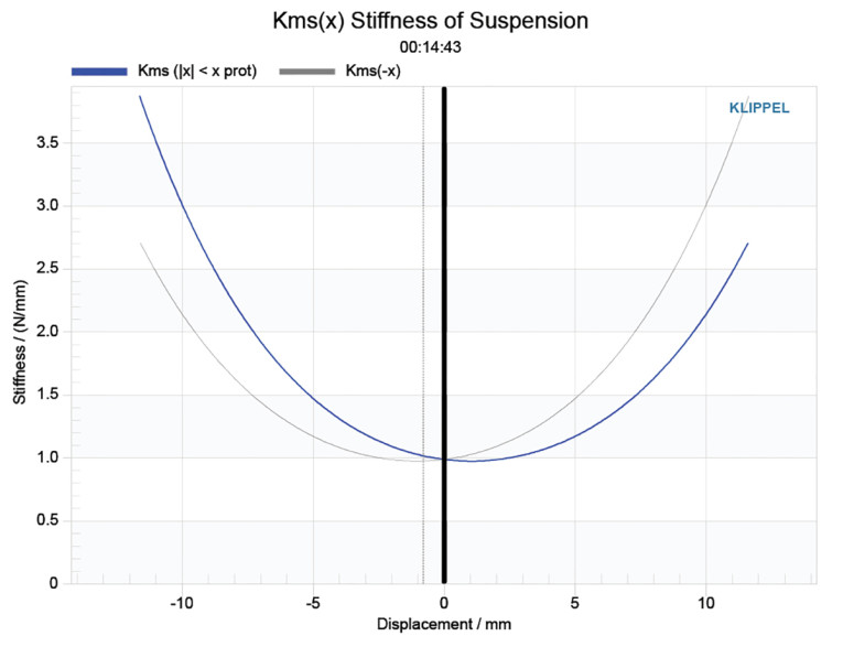
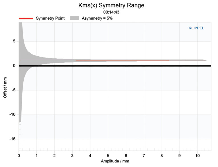
Figure 7 and Figure 8 show the Kms(X) and Kms symmetry curves for the WO24TX-4 driver. The Kms stiffness of compliance curve (Figure 7) is reasonably symmetrical and with an obvious degree of forward (coil-out) offset. The Kms symmetry range curve (Figure 8) exhibits 1mm coil-out (forward) offset at a region of high certainty (about 3mm) that remains fairly constant out to the 8.75mm physical Xmax position, where it is 1.3mm.
Displacement limiting numbers calculated by the Klippel analyzer using the full-range woofer criteria for Bl was XBl @ 82% (Bl dropping to 82% of its maximum value) equal to 8.86mm for the prescribed 10% distortion level. For the compliance, XC @ 75% Cms minimum was only 4.1mm, which means that for the SB Acoustics woofer, the compliance is the more limiting factor for getting to the 10% distortion level. If we change the criteria to the less conservative 20% distortion level, XBl goes to 10.6mm, and XC to 7.3mm.
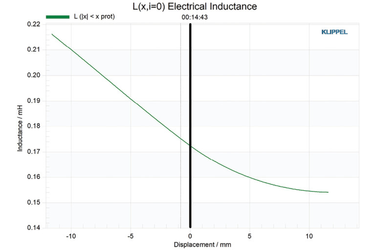
Figure 9 gives the inductance curve Le(X) for this transducer. Motor inductance will typically increase in the rear direction from the zero-rest position as the voice coil covers more of pole in a conventional motor, which is what you see in the graph. More important, the inductive “swing” from maximum inductance to minimum inductance from 8.75mm coil-in to 8.75mm coil-out varies between 0.032mH to 0.017mH, which is very good and at least in part to do the dual copper shorting rings (Faraday shield) on the undercut pole piece.
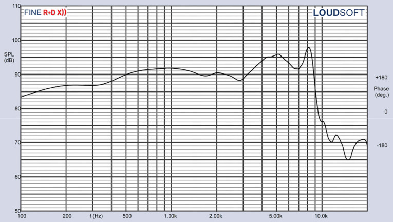
For the remaining test procedures, I mounted the SB WO24TX-4 9.5” woofer in a foam-filled enclosure that had a 19”×10” baffle and then measured the device under test (DUT) using the Loudsoft FINE R+D analyzer and the GRAS 46BE microphone (courtesy of Loudsoft and GRAS Sound & Vibration) both on- and off-axis from 200Hz to 40kHz at 2.0V/0.5m, normalized to 2.83V/1m (one of the really outstanding tricks FINE R+D can do) using the cosine windowed FFT method. All of these SPL measurements also included a 1/6 octave smoothing to approximate the 100-point LMS gated sine wave sweeps used in Test Bench for more than 20 years.
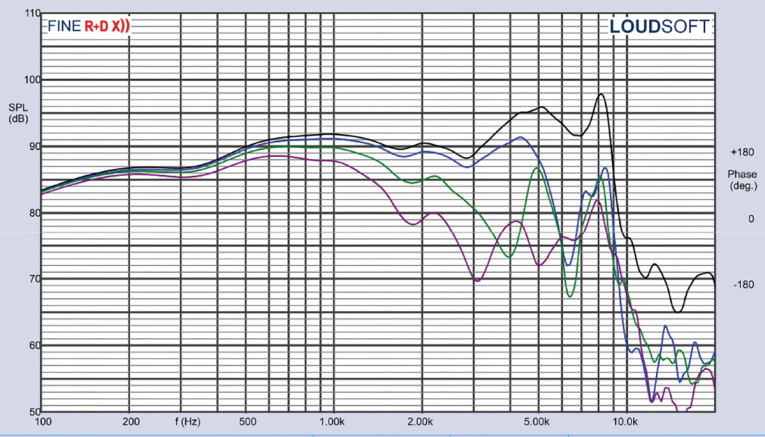
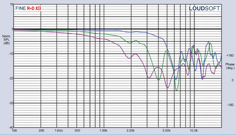
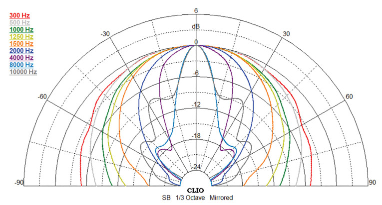
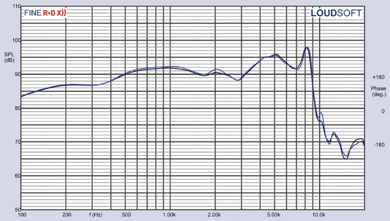
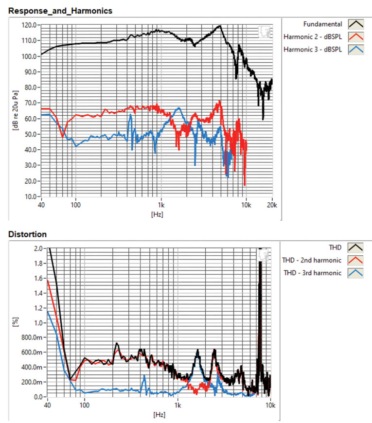
Figure 10 gives the WO24TX-4 on-axis response, indicating a fairly smooth rising response that is ±2.5dB with no break-up modes or peaking out to about 3.6kHz, with peaks in the response at 5.2kHz and 8.2kHz, beginning its low-pass roll-off. Figure 11 displays the on- and off-axis frequency response at 0°, 15°, 30°, and 45°, with -3dB at 30° with respect to the on-axis curve occurs at 1.6kHz, so a cross point in that vicinity or lower should work well to achieve a good power response (1.5kHz or lower is generally an appropriate crossover frequency for an 10” diameter woofer, and the WO24TX-4 is close to being an 10” driver). Figure 12 gives the normalized version of Figure 11, while Figure 13 displays the CLIO Pocket-generated horizontal polar plot (in 10° increments). And finally, Figure 14 gives the two-sample SPL comparisons for the WO24TX-4, showing a close match (≤0.5dB) in the operating range up to about 3kHz, except for a small area 1dB area centered on 2kHz.
For the remaining series of tests on the SB WO24TX-4, I employed the Listen SoundCheck (current version is SoundCheck 21) AudioConnect analyzer and ¼” SCM microphone (graciously supplied by the folks at Listen, Inc.) to measure distortion and generate time-frequency plots. For the distortion measurement, I mounted the 9.5” driver rigidly in free air and set the SPL to 94dB (my criteria for home audio transducers) at 1m (4.0V) using a SoundCheck pink noise stimulus.
Then, I measured the distortion measured with the Listen microphone placed 10cm from the driver. This produced the distortion curves shown in Figure 15. Note that the third-order harmonic content stays below 0.65% throughout the operating range of the driver.
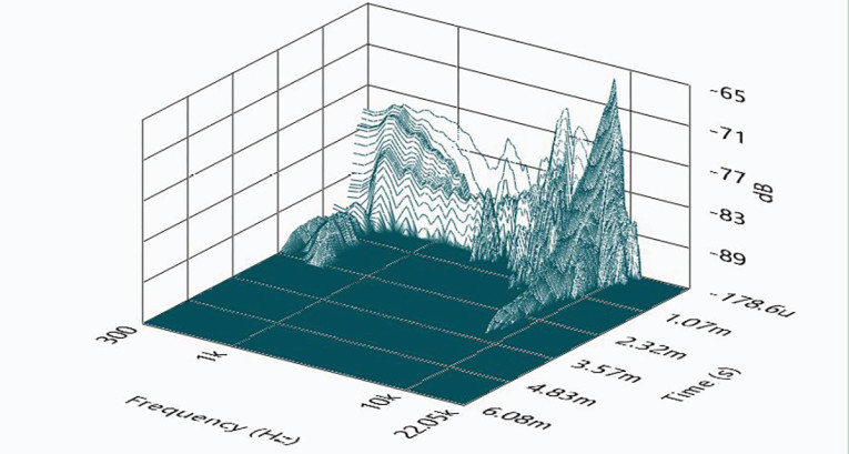
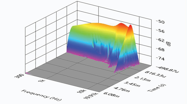
Next, I engaged the SoundCheck software to get a 2.83V/1m impulse response for this driver and imported the data into Listen’s SoundMap Time/Frequency software. The resulting cumulative spectral decay (CSD) waterfall plot is given in Figure 16, and the Wigner-Ville plot (chosen for its better low-frequency performance) is shown in Figure 17.
Combining the beneficial subjective performance of the TPCD TexTreme cone with the SB Acoustics Satori motor system makes this driver a good candidate for high-end two-channel, home theater, or studio monitor system designs. For more information, visit www.sbacoustics.com. VC
This article was originally published in Voice Coil, September 2023.