And when I attended the CEDIA Expo in San Diego, CA, in September 2017, I couldn’t ignore the staggering presence of Google and Amazon — especially Amazon. The Amazon Echo and Dot are finding serious applications in whole-house control. In fact, several education courses at the CEDIA Expo dealt exclusively with the integration of these products into home audio and control systems.
With that as inspiration, I asked the folks at Tymphany to send a couple of transducers from their Peerless by Tymphany PLS line of full-range 2” to 3” drivers. I specifically asked for the 2” PLS-50N25AL01-08 neodymium motor full range (reviewed here) as well as the 2.5” PLS-65F25AL01-08 ferrite motor full-range (reviewed separately).
The 2” PLS-50N25AL01-08
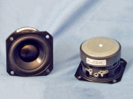
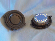
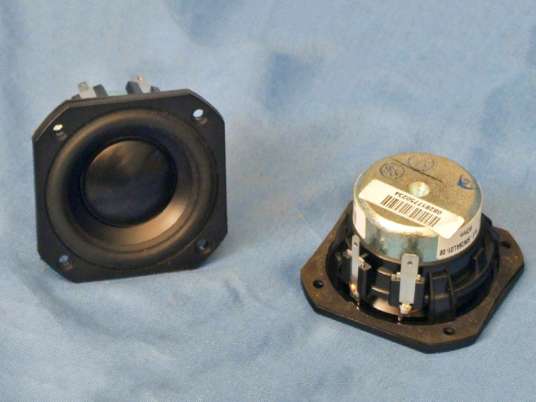
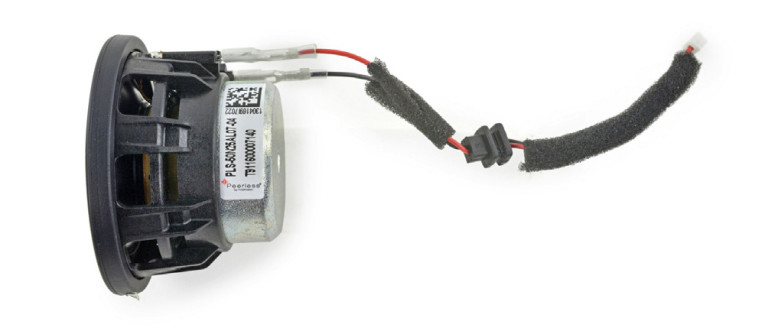
The first driver I examined was the PLS-50N25AL01-08 (see Photo 1). I chose this driver because a 4 Ω version of this driver (the PLS-50N25AL07-04) is used in the Google Home voice-activated products (see Photo 2). Feature-wise, the PLS-50N is a 2.0” diameter full-range driver built on a proprietary injection-molded polymer frame that is fully vented below the spider mounting shelf with six 3 mm × 10 mm slots for enhanced cooling. Additional cooling is provided by a series of nine 1.5 mm diameter vent holes in the 25.73 mm aluminum (ASV) former just below the neck joint. The cone assembly consists of a black anodized aluminum cone, with a 27 mm diameter aluminum dust cap (directly coupled to the 25.73 mm id voice coil former), and suspended with a NBR surround and a flat cloth spider (damper).
Powering the cone assembly is a neodymium motor with a copper cap shorting ring (Faraday shield) and a milled return cup. Tinsel leads connect on one side of the cone to a pair of solderable terminals.

I began testing the Peerless PLS-50N using the LinearX LMS analyzer and VIBox to create both voltage and admittance (current) curves. The driver was clamped to a rigid test fixture in free air at 0.3 V, 1 V, 3 V, and 6 V, with the 6 V curves remaining linear enough for LEAP 5 to get a good curve fit -impressive for a 2” driver. As has become the protocol for Test Bench testing, I no longer use a single added mass measurement. Instead, I use actual measured mass — the manufacturer’s measured Mmd data (1.57 grams).
Next, I post-processed the eight 550-point stepped sine wave sweeps for each of the PLS-50N samples and divided the voltage curves by the current curves (admittance) to produce the impedance curves — phase generated by the LMS calculation method— and imported them, along with the accompanying voltage curves, to the LEAP 5 Enclosure Shop software.
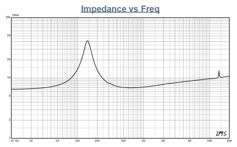
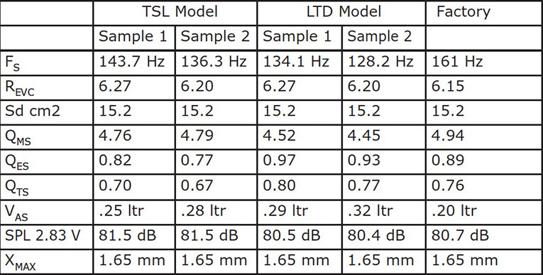
Since most Thiele-Small (T-S) data provided by OEM manufacturers is produced using either a standard method or the LEAP 4 TSL model. I additionally created a LEAP 4 TSL model using the 1 V free-air curves. I selected the complete data set, the multiple voltage impedance curves for the LTD model, and the 1 V impedance curve for the TSL model in LEAP 5’s transducer derivation menu and created the parameters for the computer box simulations. Figure 1 shows the 1 V free-air impedance curve. Table 1 compares the LEAP 5 LTD and TSL data and factory parameters for both of the PLS-50N samples. The LEAP TSL/LTD parameter calculation results for the PLS-50N was reasonably close to the factory data.
Following my usual protocol, I configured computer enclosure simulations using the LEAP LTD parameters for Sample 1. This consisted of a 61 in3 Butterworth sealed box with 50% damping material (fiberglass), and a 51 in3 Chebychev/Butterworth vented enclosure tuned to 85 Hz with 15% damping material in the box.
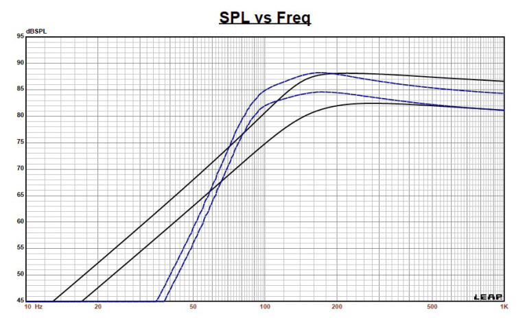
Figure 2 displays the results for the PLS-50N in the sealed and vented box simulations at 2.83 V and at a voltage level sufficiently high enough to increase cone excursion to Xmax + 15% (1.95 mm for the PLS-50N). This produced a F3 frequency of 139 Hz (F6 = 110 Hz) with a Qtc = 0.72 for the 61 in3 Butterworth sealed enclosure and –3 dB = 97 Hz (F6 = 86 Hz for the 51 in3 Chebychev / Butterworth vented simulation.
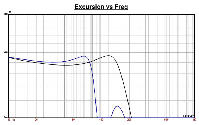
Increasing the voltage input to the simulations until the maximum linear cone excursion was reached resulted in 88 dB at 6.1 V for the sealed Butterworth enclosure simulation and 88 dB with an 4 V input level for the Chebychev/Butterworth vented enclosure. Figure 3 shows the 2.83 V group delay curves. Figure 4 shows the 6.1 V/4 V excursion curves.
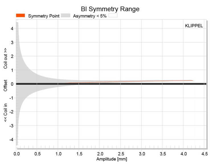

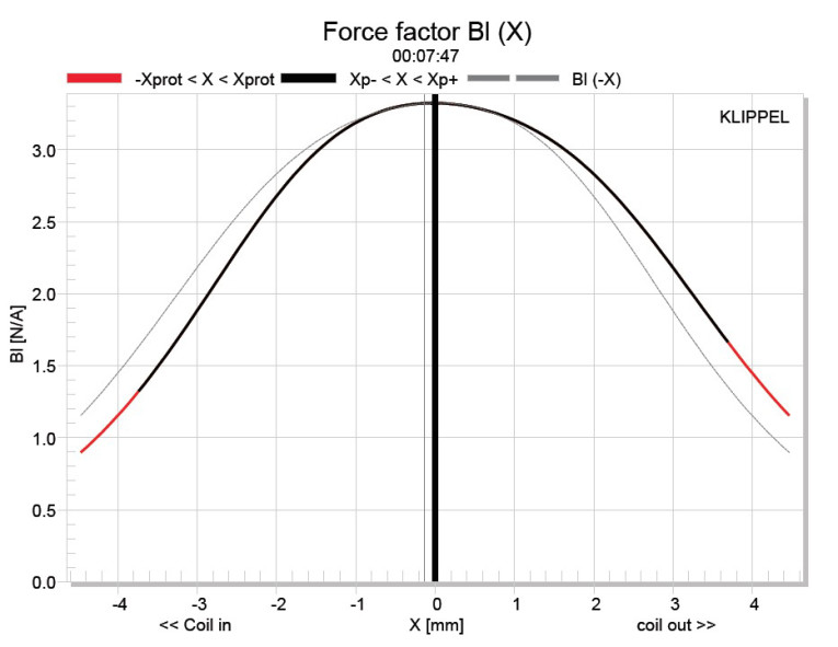
Klippel analysis for the Peerless PLS-50N 2.0” full-range produced the Bl(X), Kms(X), Bl and Kms symmetry range plots shown in Figures 5–8. For these tests, our analyzer is provided courtesy of Klippel GmbH. And, the testing is performed by Pat Turnmire, of Redrock Acoustics. (Turnmire is also the author of the SpeaD and RevSpeaD transducer design software.) The Bl(X) curve for the PLS-50N is relatively broad and symmetrical with minor amount of offset to the curve, but not bad for a short Xmax 2.0” diameter driver (see Figure 5). Looking at the Bl symmetry plot (see Figure 6), this curve shows a minor coil-out (forward) offset at the rest position (0.01 mm) that increases to a likewise trivial 0.09 mm at the driver’s physical 1.65 mm Xmax.
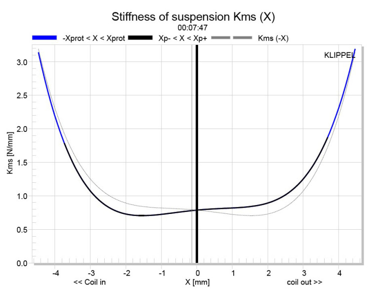
Figure 7 and Figure 8 show the Kms(X) and Kms symmetry range curves for the full-range driver. The Kms(X) curve shown in Figure 7 is also rather symmetrical, with some tilt. The curve also indicates some rearward (coil-in) offset at the Xmax position. Looking at the Kms symmetry range curve in Figure 8 shows there is about 0.75 mm at the physical Xmax position. Displacement limiting numbers calculated by the Klippel analyzer for the PLS-50N were XBl at 82% Bl is 1.9 mm and for crossover (XC) at 75% Cms minimum was 2.6 mm, which means the Bl is the most limiting factor for prescribed distortion level of 10%.
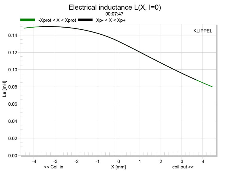
Obviously, that number is beyond the driver’s 1.65 mm Xmax so for a 2” driver, the Klippel analysis looks good. Figure 9 gives the inductance curve Le(X) for the PLS50N25AL01-08. Inductance will typically increase in the rear direction from the zero rest position as the voice coil covers more pole area. However, this device has a copper shorting ring, so the inductance variation is only 0.015 mH to 0.011 mH from the in and out Xmax positions, which is very good.
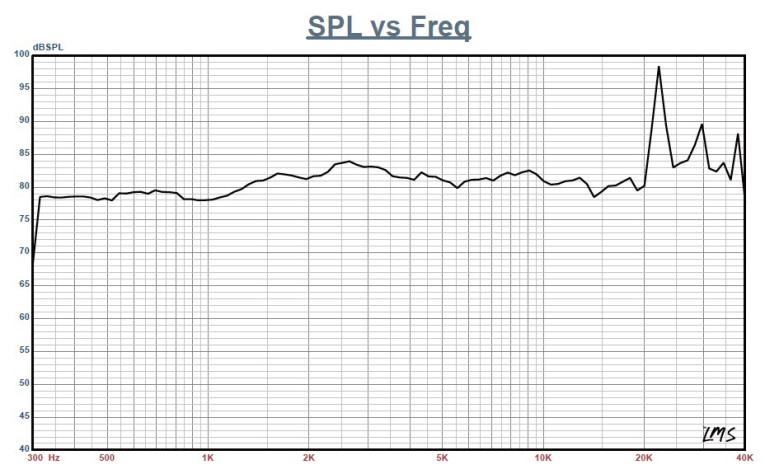
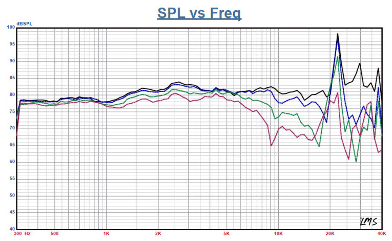

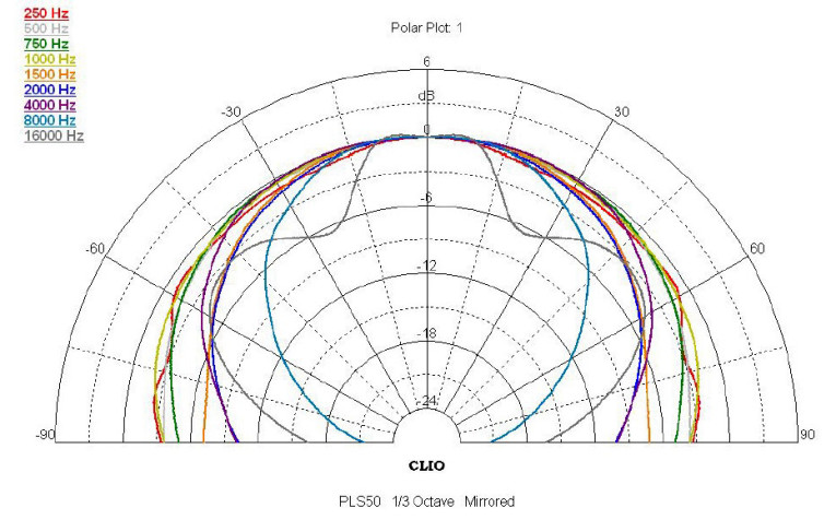
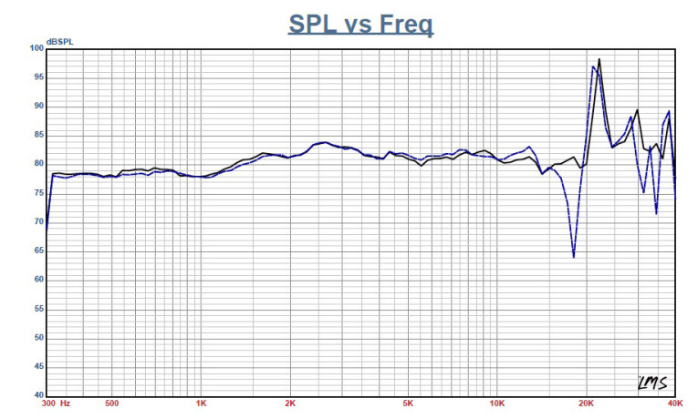
Next, I mounted the PLS-50N full-range in an enclosure, which had a 9” × 4” baffle and was filled with damping material (foam). Then, I measured the transducer on- and off-axis from 300 Hz to 40 kHz frequency response at 2.83 V/1 m using the Linear LMS analyzer set to a 100-point gated sine wave sweep. Figure 10 gives the PLS-50N ±2.9 dB (300 Hz to 20 kHz) on-axis response that is smoothly rising all the way out to 40 kHz, with the primary aluminum breakup mode at 21 kHz. Figure 11 displays the on- and off-axis frequency response at 0°, 15°, 30° and 45°.
The roll-off at 30° off axis is almost as good as a 25 mm to 30 mm dome tweeter, so I would expect the full-range fidelity of this driver to be quite good. Figure 12 gives the off-axis curves normalized to the on-axis response, with the CLIO 180° polar plot (measured in 10° increments) depicted in Figure 13. The two-sample SPL comparison is shown in Figure 14, indicating the two samples were closely matched within less than 1 dB out to 10 kHz.
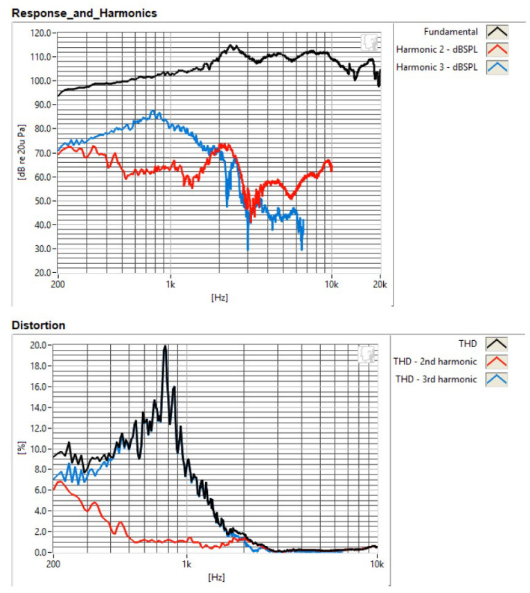

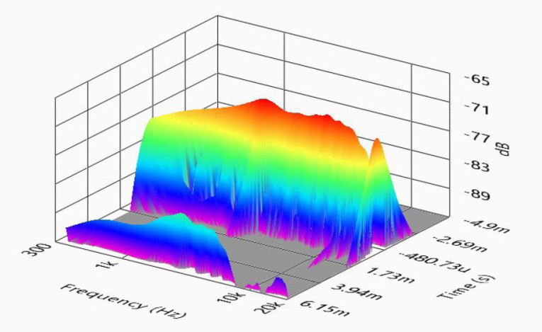
For the remaining series of tests, I employed the Listen, Inc. SoundCheck 15 software, along with the AmpConnect analyzer with the Listen 0.25” SCM microphone and power supply (courtesy of Listen, Inc.) to measure distortion and generate time-frequency plots. For the distortion measurement, I mounted the Peerless by Tymphany 2” rigidly in free air and used a noise stimulus to set the SPL to 94 dB at 1 m (6.77 V). Then, I measured the distortion with the microphone placed 10 cm from the dust cap. This produced the distortion curves shown in Figure 15. I then used SoundCheck to get a 2.83 V/1 m impulse response for this driver and imported the data into Listen’s SoundMap Time/Frequency software. Figure 16 shows the resulting CSD waterfall plot. Figure 17 shows the Wigner-Ville plot (chosen for its better low-frequency performance).
While the intended application for this Peerless 2” full-range driver is mostly TV, multimedia, and lifestyle speakers, the company also recommends it for pro sound line source applications. www.tymphany.com/peerless. VC
This article was originally published in Voice Coil, November 2017.