Simulation Techniques: Misconceptions in the Audio Industry

In this fascinating article about common sound theory misconceptions that exist in the audio and hifi communities, René Christensen debunks three of them. Starting with group delay and phase delay and why it is incorrect to say that phase and time are the same thing, what actually happens when a loudspeaker driver moves outward and inward, and the effects of polarity and phase flip. True reference material with detailed mathematical expressions and numerical analysis.
 
In the audio and hi-fi communities, some people have certain beliefs about how loudspeakers work that are demonstrably false. This article targets three of them.

“The group delay/phase delay is the ‘actual’ delay in a system.”
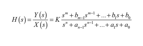
Group delay and phase delay are quantities often discussed on forums in the context of loudspeaker and subwoofer behavior, and it is evident that neither are well understood. A variation of the misconception is that “phase and time are the same thing.” Let us first look at a system and its transfer function, and then work our way toward the delays. A transfer function describes system behavior as a complex function H(s) as function of the complex frequency s [1]. It is the ratio of the output phasor Y(s) and the input phasor X(s), which are the Laplace transforms of the time signal output y(t) and the time signal input x(t), respectively. For physical systems described via linear differential equations, the transfer function is typically formulated as a rational function, meaning a function that is a fraction with a polynomial in the numerator and a polynomial in the denominator. The transfer function directly tells us a particular behavior of the system, namely its steady-state behavior. There is an associated frequency response, which consists of a magnitude response and a phase response. These responses focus on the subset of frequencies that fall on our “standard” frequency line, where the sinusoids reside. While the general transfer function also directly gives us the response for exponentially damped or increasing sinusoids, the sinusoidal response will typically suffice to describe the system, as any relevant music can be decomposed into such sinusoids. The magnitude response is not important for the delays as they are calculated from the phase response, which can be expressed as:
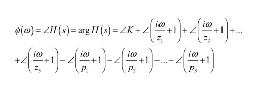
The zs indicate the zeros of the transfer function, meaning the solutions to the denominator polynomials, and the ps are the poles; the solutions to the numerator polynomial. When the phase response has been established, two relevant delays can be calculated, the phase delay t_p and the group delay t_g: Before going into too many details, it can be informative to illustrate how to think about these delays. The phase delay can be found by drawing a straight line from any frequency in question to the (0,0) point and finding the negative slope of said line to arrive at a time value. Similarly, the group delay is found via a negative slope, but here it is the local slope of the phase calculated via the derivative. The major point to note about these delays are that they are defined via the phase, and since phase is defined for steady-state conditions only, the delays are also limited to steady-state behavior. So while, for example, the group delay can be negative in part of the frequency range, that does not indicate any issues with causality in general.

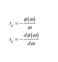
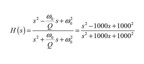
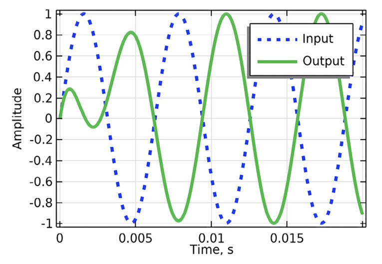
For the special case of a linear phase, the phase delay and the group delay have the same value across all frequencies, and this case is a “pure” time delay, which we will discuss a little later. In general, however, the phase delay will indicate the apparent delay in the system when viewed at steady-state, and the group delay will indicate how the envelope of a group of frequencies around a certain frequency will appear delayed. But there might not be any latency in the system at a frequency, where both phase delay and group delay are non-zero, as we can illustrate with a second-order allpass filter transfer function with Q=1 and ω0=1000 rad/s (i.e., a frequency of 159Hz): The phase of this transfer function is plotted alongside the phase and group delays in Figure 1, and at the characteristic frequency ω0 these delays are clearly non-zero.
 
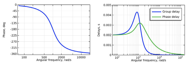
But if we calculate the output including the transient response at this frequency for a sinusoidal input as illustrated in Figure 2, we see clearly that there is an immediate output, so there is zero inherent latency in the system at this frequency. The phase delay does indeed match up with the apparent delay seen between the input and the output after steady state is reached, but the group delay only gives an indication as to when the transient response settles into steady state, and its actual value does not indicate any “true” delay in the output. Phase delay and group delay need to be considered as a pair, and as we will see later, their differential is important. They are always be derived from the steady-state phase, but this phase cannot in general be derived from any one of them, and neither one of them generally reveal the transient delay directly without some explicit calculations. Hence, it is also incorrect to say that phase and time are the same thing.
 
“A loudspeaker driver works by creating a high pressure as it moves outward, and a low pressure as it moves inward.”
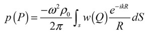
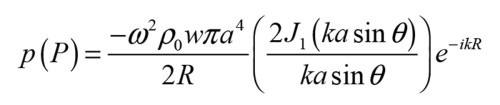
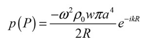
This is one of the most significant misbeliefs that I see repeated often, as it is completely opposite to how the sound from a loudspeaker is generally generated. Let us first set the stage: We are looking at steady-state conditions where the system has had time to settle and simple oscillation is achieved, which is how we analyze loudspeakers most of the time. For each frequency we look at how the driver is moving and compare it to the resulting pressure. And we are looking at anechoic conditions, so there is no room to consider. This situation can of course be modeled, and the perfect place to start is with the so-called First Rayleigh Integral [2], where the pressure phasor is calculated as: The integral gives us exactly the complex pressure p in point P at a distance R from a point Q on a vibrating flat surface with an outward displacement w(Q) possible varying over the piston surface S under free-field conditions, and we can immediately note a minus sign being present on the righthand side of the equation. This indicates that there is a general sign change between displacement (seen as being positive moving outward from equilibrium) and the resulting pressure (seen as positive under compression). We can simplify the expression by assuming a circular piston, a constant displacement across the piston, and that the measurement point P is in the far-field relative to the radius a of the piston with R>>a, giving a pressure of: Furthermore, if the measurement point is located on-axis with θ=0, the expression in the parentheses equals one, and the pressure simplifies to: The exponential term accounts for the phase related to the time it takes for the waves to travel from the piston to the measurement point, and that phase is typically ignored in measurements by subtracting it from the total phase to get to the relevant phase of the pressure related to the system behavior. With an inherent vector direction being positive outwards from the piston to the exterior domain in front of it, the pressure phasor is in anti-phase with the displacement phasor, whereas the acceleration phasor of the piston is in-phase with the displacement phasor. As the piston reaches its outermost position achieving its maximum positive displacement, the sound pressure is at its lowest negative value, meaning maximum rarefaction is achieved, as opposed to maximum compression. At this position, the piston acceleration will have reached its lowest negative value for its acceleration phasor, and in general the pressure phase and level will correlate well with the acceleration dittos.

Instead of an analytical expression, we can also do a numerical analysis with the simulation software COMSOL Multiphysics. A circular piston is placed in an infinite baffle, and an enclosure is placed behind the piston as shown in Figure 3.
 
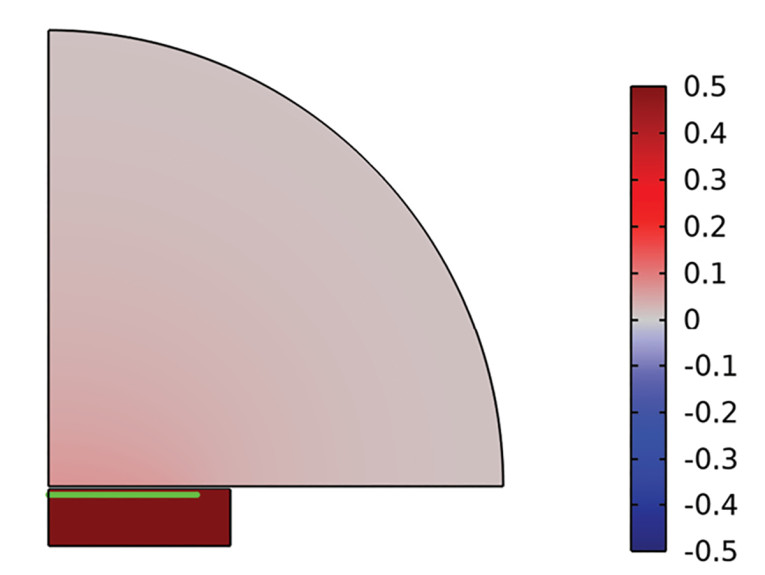
We can see from the color legend that at its most inward position, the piston compresses the air in the enclosure on its rear side, as well as the air on its front, so a positive sound pressure is seen on either side. This goes against the common belief that the exterior sound pressure should be at its highest positive value in the most outward position of the piston.

The enclosure pressure illustrates where this wrong intuition might come from, as here we do indeed see the displacement being in-phase with the pressure due the acoustical impedance being a compliance and not free-field conditions. In general, the resulting pressure phase will not only depend on the phase of the piston displacement, but also on the phase of the acoustic impedance that describes the acoustic environment in question.

If a loudspeaker worked by creating compression air as its cone moves outwards from its equilibrium, all our textbooks would have to be rewritten, and our definition of correct polarity would need a flip. Speaking of polarity flip…


“A polarity flip cannot be equivalent to a 180° phase shift, since such a phase shift would entail a time delay.”
This is a classic on Hi-Fi forums and has been for years. A polarity flip is what you get when you flip your loudspeaker wires, on both left and right speakers, so that the “red” wire goes to “black” terminal and vice versa. The resulting displacement on the cone will now be opposite of what it would otherwise; an inward displacement now becomes an outwards displacement. We can describe the polarity flip as a system with the following transfer function: A transfer function is generally a complex valued function and here the argument is the complex frequency s=σ+iω. From the transfer function we can derive the system’s magnitude and phase responses. The magnitude response is the same as that of a wire, as magnitude is unaffected by a sign change, so we get: With the magnitude unaltered, a polarity flip must then change the phase, and indeed it does. Starting out with Euler’s identity we can see how a complex exponential with a phase of φ can be written via trigonometric functions as: To arrive at a value of minus one, we set the phase to π radians or 180°:
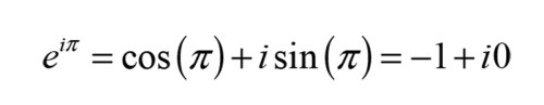
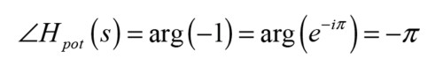
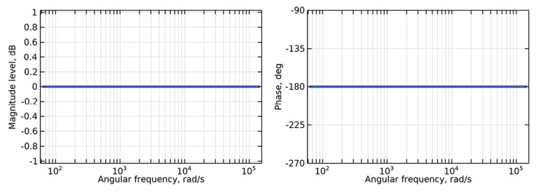
The 180° might as well be written as -180° as these two phases coincide, and the latter is the choice typically made when looking at transfer functions, ending up with the phasor phase associated with a polarity flip being minus −π radians at all frequencies as: So, the effect of a polarity flip can be visualized via its frequency response shown in Figure 4.
 
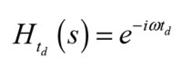
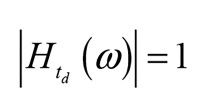
Now, what can be confusing is that other transfer functions can have a 180° phase shift at certain frequencies, and they will have the same steady-state output, assuming of course they share the same magnitude response value, at those frequencies. One such transfer function is that of a pure time delay. All the delay does is… well, delay the output. So any input will “buffered” in some sense before being output, which could be achieved with a digital system or via a transport delay where the signal is taken out of a wave at a distance from some input source. It could be also to some degree be approximated via a high-order Bessel allpass function [3]. The time delay constitutes a so-called “distortionless system” [1], as it has a magnitude response of one and a linear phase leading to no magnitude distortion and no phase distortion. The transfer function for a time delay of td seconds is: And the magnitude response and phase response are, respectively:
And:  The responses are plotted in Figure 5.
 
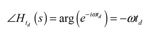
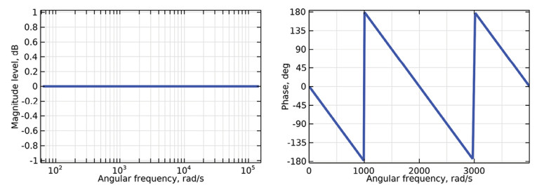
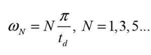
Where a polarity flip has a phase of -180 degrees at all frequencies, we see that the time delay will only have a phase shift of -180° at some discrete (angular) frequencies, namely at: At these frequencies the time delay system will have a delay that fits with half a period, T/2, so at steady state the phase delay will be the same as for the polarity flip. If you look at the steady-state outputs from the two systems at one of those frequencies, there is no way to distinguish the polarity flip from the time delay. But we could make infinitely many systems that at these frequencies will have the same steady-state output as these two systems. What we need to remember is that there also is a transient response to consider, and here we will immediately see the difference. In Figure 6, three signals are shown — an input signal, the output from a polarity flip, and the output from a time delay at a frequency where the two systems have the same phase of 180°. It is clearly seen that the two outputs are not the same in the beginning but then look indistinguishable after half a period.
 
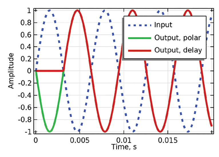
Not only do the two systems have different phase responses, but even for the few frequencies where they do happen to have the same phase, and hence phase delay, and share the same steady-state response, they can never have the same transient response. A major issue can be seen now, and that is that if you start from a drawing of an acausal/steady-state sinusoidal input and ditto output, you entirely miss which type of system caused the output you are looking at and what the associated transient behavior is. So, you cannot start from the output signal and work your way back to the system — you need to work from the system to the output signal.

One thing to note is that the polarity flip will have an associated phase delay that increases to infinity at low frequencies, as the apparent delay needed time for the steady-state response to look like that of the polarity flip will increase toward low frequencies as the slope drawn down to the phase value will increase. At low frequencies the period is long, and so a substantial time delay would be needed to achieve a 180° phase shift via a time delay of half a period.

But this is just an abstraction, and not a true delay. The polarity flip and other phase ambiguities can make it tricky to even plot the phase delay, compared to the group delay. The group delay of the polarity flip is zero, whereas both the phase delay and the group delay for the time delay system are equal to the time delay itself.

In conclusion, a polarity flipped signal has no inherent time delay, and the output will only look like a time-delayed version of the input when viewed steady-state. But that goes for any other output signal with a phase different than that of input signal, hence our calling the phase delay, and group delay for that matter, “apparent” delays [4]. The allpass filter discussed earlier is seen to also have the same steady-state response at the chosen frequency, and so shares the phase and phase delay, with the other two systems at this frequency, but with a different group delay again and different transient behavior.

Conclusion
The article has gone through some essential topics in signal processing and loudspeaker analysis. In an upcoming article, I will go through phase and delay aspects related to loudspeakers in more detail. aX


References
[1] A. B. Carlson, Communication Systems: An Introduction to Signals and Noise in Electrical Communication, Singapore: McGraw-Hill, 1986.
[2] L. E. Kinsler, A. R. Frey, A. B. Coppens, and J. V. Sanders, Fundamentals of Acoustics, Danvers, Massachusetts: Wiley, 2000.
[3] R. Christensen, “#039: Allpass Systems: Phase and Time Delay,” Acculution, April 23, 2022,
www.acculution.com/single-post/039-allpass-phase-and-time-delay
[4] M. W. J. Leach, “The Differential Time-Delay Distortion and Differential Phase-Shift Distortion as Measures of Phase Linearity,” Journal of the Audio Engineering Society (JAES), Volume 37, No. 9, pp. 709-715, 1989.

This article was originally published in audioXpress, June 2023