Unquestionably, the 2” to 2.5” diameter full-range drivers are one of the most used transducers in consumer electronics. They are finding broad use in soundbars, pedestal soundbars (soundbars that contain down firing subwoofers that double as TV stands), docking stations (these are starting to go away), and desktop speakers such as the Sonos products, and portable Bluetooth speakers (e.g., Jambox, Beats, Samsung, Bose, and a million others). Indonesian-based SB Acoustics sent its entry into this crowded field of play, the new SB65WBAC25-4 (see Photo 1).
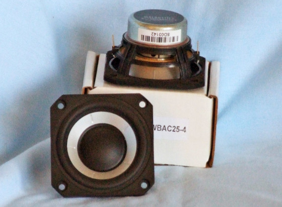
The SB65WBAC25-4 is a 2.5” diameter full-range driver built on a proprietary injection-molded polymer frame that is fully vented below the spider mounting shelf for enhanced cooling. The cone assembly consists of a “dented” aluminum cone. The “dents” were added to improve stiffness, with a 30-mm diameter plastic dust cap, suspended with a NBR surround and a flat cloth spider (damper). For a 2.5” woofer, the SB65WBAC25-4 has a rather large 25.4-mm diameter voice coil wound with round copper wire on a nonconducting vented former, terminated on opposite sides of the cone to solderable gold-plated terminals. Driving the cone assembly is a neodymium motor using a neodymium ring magnet rather than a slug, and a milled return cup.
I used the LinearX LMS analyzer and VIBox to create both voltage and admittance (current) curves with the driver clamped to a rigid test fixture in free air at 0.3, 1, 3, and 6 V. I discarded the 6-V curves as being too nonlinear for LEAP 5 to get a good curve fit. As has become the protocol for Test Bench testing, I no longer use a single added mass measurement. Instead, I use actual measured mass, and the manufacturer’s measured Mmd data (2.45 grams).
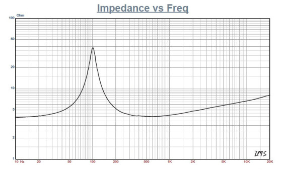
Next, I post processed the six 550-point stepped sine wave sweeps for each of the SB65WBAC25-4 samples and divided the voltage curves by the current curves (admittance) to produce the impedance curves, phase generated by the LMS calculation method. I imported them, along with the accompanying voltage curves, to the LEAP 5 Enclosure Shop software. Since most T-S data provided by OEM manufacturers is produced using either a standard method or the LEAP 4 TSL model, I used 1-V free-air curves to additionally create a LEAP 4 TSL model. I selected the complete data set, the LTD model’s multiple voltage impedance curves, and the TSL model’s 1-V impedance curve in LEAP 5’s transducer derivation menu. Then, I created the parameters for the computer box simulations. Figure 1 shows the 1-V free-air impedance curve. Table 1 compares the LEAP 5 LTD, the TSL data, and the factory parameters for both of the SB65WBAC25-4 samples.
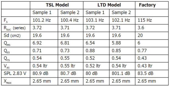
LEAP TSL parameter calculation results for the SB65WBAC25-4 were reasonably close to the factory data. However, the QTS for the LTD multi-voltage parameters exhibited a somewhat higher number. Next, I followed my usual protocol and used the LEAP LTD parameters for Sample 1 to set up computer enclosure simulations. I programmed two vented enclosure simulations into LEAP—an 89-in3 Chebychev / Butterworth-type vented alignment tuned to 65 Hz (with 15% damping material) and a 63-in3 vented enhanced Q Butterworth alignment (with 15% damping material in the box) tuned to 103 Hz.
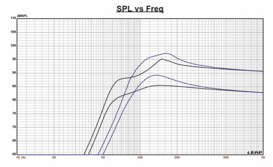
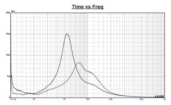

Figure 2 shows the SB65WBAC25-4’s results in the two vented box simulations at 2.83 V and at a voltage level sufficiently high enough to increase cone excursion to 3 mm (XMAX + 15%). This produced a F3 frequency of 80.7 Hz (F6 = 60 Hz) for the 89-in3 Chebychev / Butterworth enclosure and –3 dB = 102 Hz for the 63-in3 enhanced Q Butterworth vented simulation. Increasing the voltage input to the simulations until reaching the maximum linear cone excursion resulted in 95 dB at 18 V for the Chebychev / Butterworth enclosure simulation and 97 dB with an 8-V input level for the enhanced Q Butterworth vented enclosure. Figure 3 shows 2.83-V group delay curves. Figure 4 shows the 8-V excursion curves.
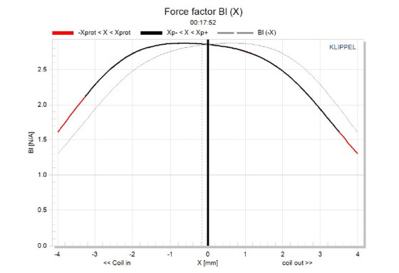
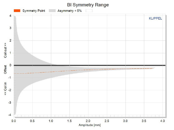
The SB65WBAC25-4’s Klippel analysis produced the Bl(X), KMS(X), and Bl and KMS symmetry range plots shown in Figures 5–8. Figure 5 shows the SB65WBAC25-4’s Bl(X) curve is relatively broad and fairly symmetrical with some “tilt” to the curve, but not bad for a short XMAX 2.5” diameter driver. Figure 6 shows the Bl symmetry plot with a minor coil-in (rearward) offset at the rest position that decreases to 0.29 mm at the driver’s physical 2.65-mm XMAX.
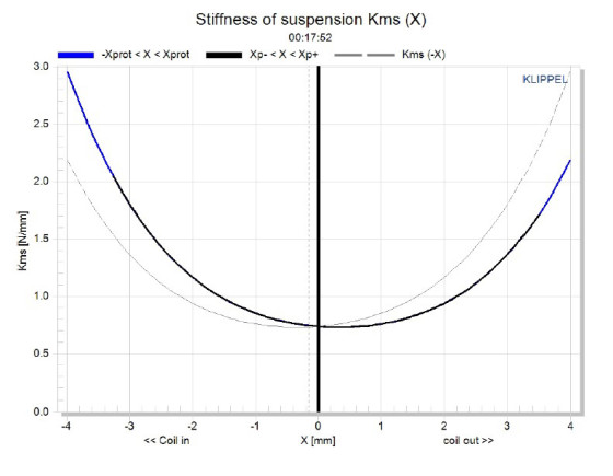
Figure 7 and Figure 8 show the KMS(X) and KMS symmetry range curves. The KMS(X) curve is also moderately symmetrical and has a very minor forward (coil-out) offset at the rest position, staying mostly constant to about 0.36 mm at the physical XMAX position. The SB65WBAC25-4’s displacement limiting numbers were XBl at 82% (Bl is 2.9 mm) and for XC at 75%, CMS minimum was 2.6 mm, which means that compliance is the most limiting factor for a prescribed distortion level of 10%.
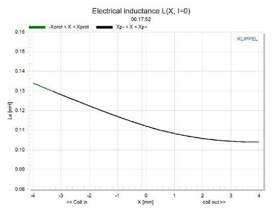
Figure 9 shows the SB65WBAC25-4’s inductance curve Le(X). Inductance will typically increase in the rear direction from the zero rest position as the voice coil covers more pole area, which is what happens. However, the SB65WBAC25-4’s inductance variation is only 0.014 to 0.007 mH from the in and out XMAX positions, which is very good.

Next, I mounted the SB65WBAC25-4 in an enclosure that had a 9”× 4” baffle filled with damping material (foam). Then, I used the LinearX LMS analyzer set to a 100-point gated sine wave sweep and measured the transducer on and off axis from a 300-Hz-to-40-kHz frequency response at 2.83 V/1 m.
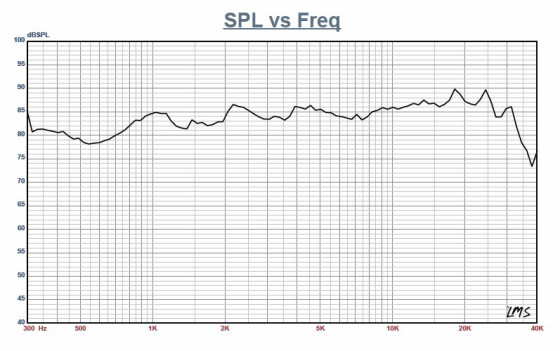
Figure 10 shows the SB65WBAC25-4’s on-axis response, indicating a smoothly rising response all the way out to 30 kHz. The big mistake I think a lot of designers make is not to equalize the upper rise. If you don’t, it makes the speaker sound thin and really lacking bottom end. The trade-off, of course, is that the device’s apparent loudness decreases. One way to overcome that issue in these small two-driver Bluetooth devices—ones that have the woofers mounted close together with no possibility of any stereo phantom center—is to drive them in parallel as a mono source, thus increasing the product efficiency by 3 dB.
Figure 11 displays the on- and off-axis frequency response at 0°, 15°, 30°, and 45°. The roll-off at 30° off axis is almost as good as a 25–30 dome tweeter, so I would expect this driver’s full-range fidelity to be quite good. Figure 12 shows the SB65WBAC25-4’s two sample SPL comparison, which is a close match to within less than 0.5 to 1 dB throughout the operating range.

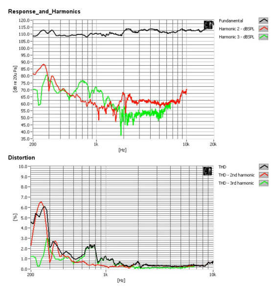
For the remaining tests, I used the Listen SoundCheck AmpConnect analyzer with the Listen 0.25” SCM microphone and power supply to measure distortion and generate time-frequency plots. For the distortion measurement, I rigidly mounted the SB65WBAC25-4 in free air and used a noise stimulus to set the SPL to 94 dB at 1 m (7.2 V). Then, I measured the distortion with the microphone placed 10 cm from the dust cap.
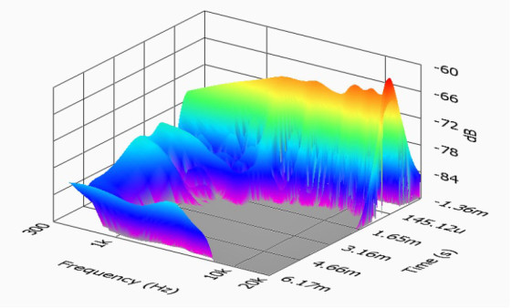
Figure 13 shows the distortion curves. I then used SoundCheck to get a 2.83-V/1-m impulse response and imported the data into Listen’s SoundMap Time / Frequency software. Figure 14 shows the resulting CSD waterfall plot. Figure 15 shows the Wigner-Ville plot. While the intended application for this SB65WBAC25-4 is TV, multimedia, and lifestyle speakers I suggest it would make a great driver for line-source applications.
www.sbacoustics.com


This article was originally published in Voice Coil, January 2015