Short after the European COMSOL Conference 2023 held in Munich, Germany, from October 25-27, and which signaled the return of in-person events for the company, the excitement about the upcoming COMSOL Multiphysics release was building up. With some of the new features already publicly discussed and creating excitement, it was clear that the COMSOL development team didn't want to hold any longer what they have been working on for some time.
COMSOL Multiphysics version 6.2 is a very significant update that reflects the intense momentum around its global user base, pushing modeling and simulation applications to the limit almost daily. Naturally, these interactions are reflected in the latest version of the multiphysics simulation software, which also speeds up computations in multiple ways.
The latest version of COMSOL Multiphysics solidifies its standing as a comprehensive multiphysics simulation software, offering unmatched physics modeling and simulation capabilities within a single software environment. It also enhances its support for building, maintaining, and compiling standalone simulation apps, thereby extending the use of simulation to individuals beyond the modeling and simulation community.
The software update features high-performance multiphysics solvers for the analysis of electric motors, up to 40% faster turbulent CFD simulations, and an order of magnitude faster impulse response calculations for room and cabin acoustics. Additionally, it is now up to 7 times faster to perform boundary element analysis (BEM) for acoustics and electromagnetics when running on clusters.
Effective Simulation Apps and Digital Twins
Surrogate models deliver accurate simulation results much faster than the full-fledged finite element models that they approximate. When used in simulation apps, this leads to near-instantaneous results, providing app users with an improved interactive experience. In addition, surrogate models are useful for digital twins, where fast and frequent updates of simulation results are often necessary.
The latest COMSOL Multiphysics software version 6.2 also introduces the ability to make simulation apps with automated updates through timer events, which is especially useful when creating digital twins or IoT-connected simulation apps.
"Surrogate models significantly strengthen the app-building capabilities in COMSOL Multiphysics, and open up new possibilities to our users," says Lars Langemyr, chief scientist at COMSOL. "They can now create effective digital twins and build interactive, computationally fast, and accurate standalone apps."
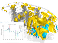
Version 6.2 expands the capabilities for efficient simulation of electric motors as well as for transformers and other electric machinery through a time periodic solver, available in the AC/DC Module. It also enables multiphysics motor analysis involving acoustics, structural mechanics, multibody dynamics, and heat transfer, and makes it possible to run optimization studies to find new motor designs.
"The new solving method makes an important class of electric motor simulations several orders of magnitude faster," says Durk de Vries, technical product manager for the AC/DC Module at COMSOL. "It allows for efficient analysis of multiphysics phenomena that were previously out of reach. This is pivotal for electric motor design optimization, where a balance between structural, thermal, and electromagnetic objectives is essential."
In version 6.2, users will discover new modeling features across the board. Core offerings, like visualization and meshing, are improved, and add-on products are expanded and updated. Version 6.2 also adds more than 100 new and updated example models, helping users enhance their modeling skills.
Some highlights from the broadened scope of physics modeling include realistic frequency-dependent materials for acoustics simulations in the time domain, extended damage, fracture, and contact modeling, easy-to-use specific absorption computations for RF tissue simulations, analysis of light propagation through liquid crystals, and the bility to use local weather data for temperature and pressure in simulations, based on a GPS location, among others.
COMSOL Multiphysics simulation software is able to expand to electromagnetics, structural, acoustics, fluid flow, heat transfer, and chemical applications. With COMSOL Multiphysics version 6.2, the company significantly expanded the features supported by the Acoustics Module, which is undoubtedly one of its most popular, and fast-expanding application segments.
Version 6.2 introduces a new frequency-dependent Impedance condition for time-domain pressure acoustics, a new anisotropic material model in the Poroelastic Waves interface, and a new Port boundary condition for enhanced modeling of aeroacoustics based on linearized potential flow. The list of new tools and features is extensive, and COMSOL provided various examples and tutorials that illustrate what is possible. Here are some of the highlights.
For the Pressure Acoustics, Transient interface and the Pressure Acoustics, Time Explicit interface, there is new functionality for specifying and setting up frequency-dependent impedance conditions in the time domain. The functionality provides a rational approximation of the frequency-domain data, resulting in a system of ordinary differential equations (memory equations for the inverse Fourier transform) solved in the time domain.
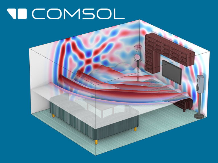
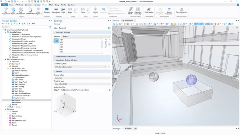
A new function for fitting or interpolation has also been added to perform the transformation from the frequency-domain data to the time domain, where the fitting relies on a variant of the adaptive Antoulas–Anderson (AAA) algorithm. This new functionality is showcased in the updated Wave-Based Time-Domain Room Acoustics with Frequency-Dependent Impedance tutorial model.
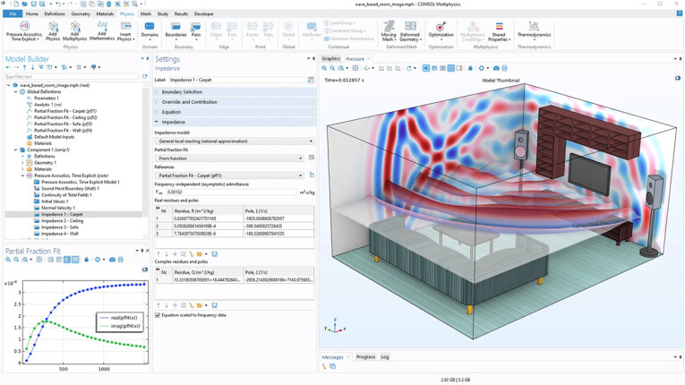
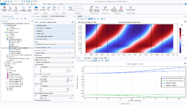
The Impedance boundary condition in the Pressure Acoustics, Transient and Pressure Acoustics, Time Explicit interfaces can now be used to model realistic surface properties, such as those of an absorbing panel or any other surface that has frequency-dependent absorbing properties. There are two new options available, Serial coupling RCL and General local reacting (rational approximation), the latter of which relies on a special transformation of the surface impedance data, which can be achieved with the new Partial Fraction Fit function. This new functionality is essential when modeling, for example, realistic wave-based room acoustics simulations in the time domain.
The Partial Fraction Fit function transforms frequency-domain data into a form that is suitable for a time-domain analysis. The function performs a rational approximation of frequency-domain responses. This makes it possible to compute its inverse Fourier transform analytically and thus obtain the time-domain impulse response function. The fitting algorithm can be used for any data, but it is particularly important and useful for surface impedance data in acoustics simulations.
The Impedance boundary condition in the Pressure Acoustics, Time Explicit interface. The necessary data for the General local reacting (rational approximation) condition is directly imported from the Partial Fraction Fit function that fits the frequency-domain admittance.
The Poroelastic Waves interface has been extended to include a new material model, Anisotropic Poroelastic Material. Many porous materials, like fibrous materials, exhibit anisotropic properties. The anisotropic properties can now be defined for the elastic matrix material properties as well as the relevant poroacoustic properties; that is, the flow resistivity, the tortuosity factor, and the viscous characteristic length.
Multiphysics Couplings
The Acoustic FEM–BEM Boundary coupling and the Acoustic–Structure Boundary coupling now include the option to add subfeatures, and two new multiphysics couplings have been added to the Acoustics Module to simplify the modeling workflow. An example is the new boundary pair version of the previously available Acoustic–Thermoviscous Acoustics Boundary coupling. This coupling is suited for modeling assemblies with nonconforming meshes. When coupling pressure acoustics models based on the finite element method (FEM) and boundary element method (BEM) using the Acoustic FEM–BEM Boundary multiphysics coupling, an impedance subfeature can now be added between the two domains. This extends the use of the hybrid FEM–BEM modeling strategy, which is useful for large acoustical problems.
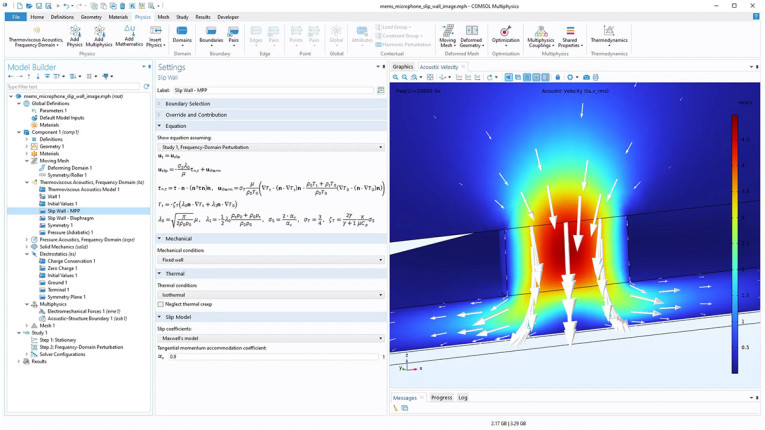
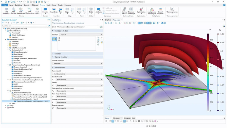
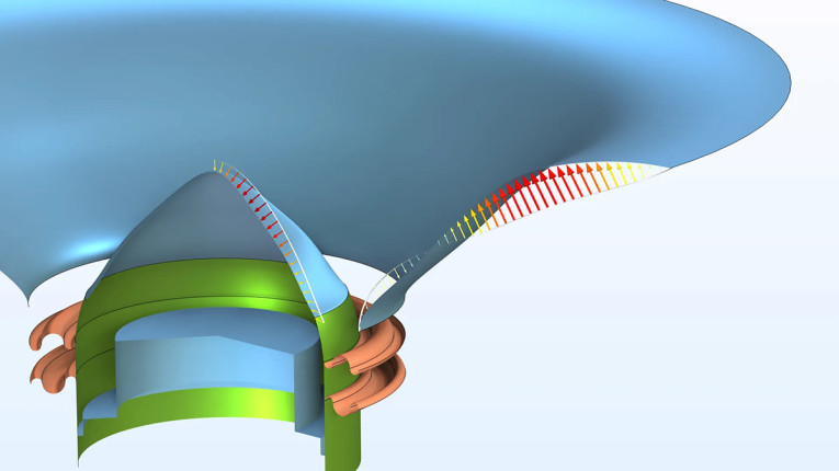
When coupling a vibrating structure to an acoustic domain using the Acoustic–Structure Boundary multiphysics coupling, a Thermoviscous Boundary Layer Impedance subfeature can be added to the multiphysics coupling. This simplifies the setup of large vibroacoustic models where thermoviscous losses are included with the homogenized boundary condition formulation of the thermoviscous boundary layer impedance. This functionality is also important for speeding up certain shape optimization problems, or for faster approximate simulations. This new addition is illustrated in the Piezoelectric MEMS Speaker tutorial model.
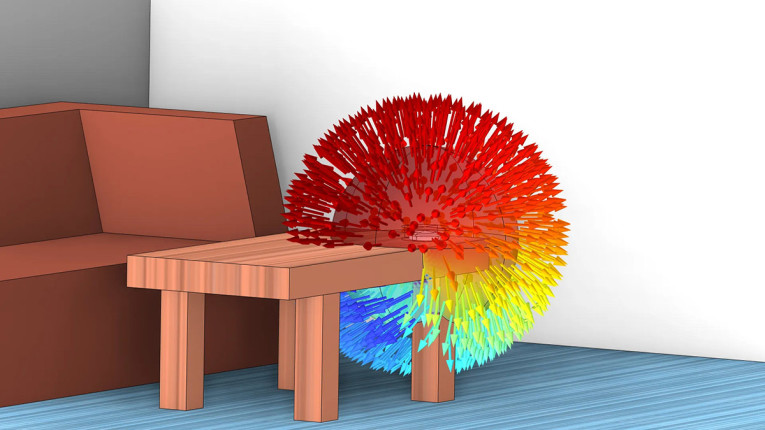
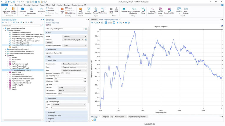
For the data source for the Impulse Response plot, there is now a Function option (as opposed to only a receiver dataset). This means that the Impulse Response plot can be used to analyze user-defined impulse response data, for example, based on a WAV audio file import. This functionality enables the analysis of measurement data as well as data resulting from a concatenation of low-frequency wave-based and high-frequency ray simulations.
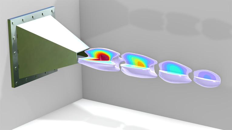
Gradient-based optimization (shape or topology optimization) is now supported in 2D axisymmetric models when using the dedicated optimization exterior-field Lp_pext_opt operator in the Pressure Acoustics, Frequency Domain interface. The optimization version of the exterior field operator, similar to the already existing operator in 3D, is implemented such that its sensitivity can be computed analytically. As an example, the Tweeter Dome and Waveguide Shape Optimization tutorial model has been updated to use the new operator, and the acoustic domain can now be highly reduced and the model runs 50% faster. This update is also illustrated in the Optimizing the Shape of a Horn tutorial model.
A new frequency-domain study type called Adaptive Frequency Sweep has been added to the Pressure Acoustics, Frequency Domain interface. The study is useful for performing dense frequency sweeps in an efficient manner using the asymptotic waveform evaluation (AWE) method.
Users can now perform analyses of vibroacoustic multiphysics models using the modal solver. This is made possible since both the left and right eigenvectors are now computed when performing an eigenfrequency analysis. This functionality is shown in the Acoustic–Structure Interaction with Frequency Domain, Modal Solver tutorial model.
Several important improvements have also been introduced for when solving acoustic models with the boundary element method (BEM) using the Pressure Acoustics, Boundary Elements interface.
The COMSOL website provides the full list of new features, enhancements, and improvements, with direct links to the new and updated tutorials, which includes a full frequency-domain analysis of a 3D vibroelectroacoustic multiphysics model of a loudspeaker, among many other examples.
www.comsol.com