As it happens every year, immediately after or during its annual conference, COMSOL announces the latest update to its integrated software suite. A leading 3D modeling and simulation environment for product design and research, COMSOL Multiphysics is currently the global standard in many market specific applications, including acoustics, fluids, heat transfer, and chemical applications, which can be interfaced also with all major technical computing and CAD tools on the CAE market.
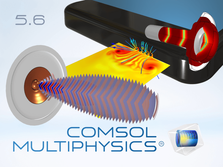
With the latest release of COMSOL Multiphysics version 5.6, the company significantly expands the number of functionalities, tools and features, including its Acoustics Module, which currently is powering development efforts across all segments of the audio industry, from speaker and transducer design to cutting-edge acoustic metamaterials.
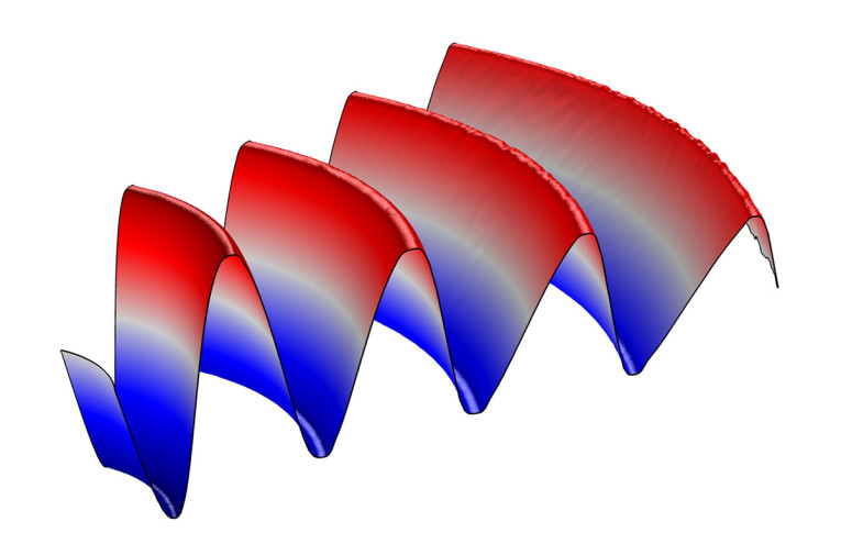
Included in the Acoustics Module of COMSOL Multiphysics version 5.6, are new Nonlinear Pressure Acoustics, a new Time Explicit physics interface and Nonlinear Thermoviscous Acoustics Contributions. The former is based on dG-FEM and designed for modeling progressive propagation of finite-amplitude nonlinear acoustic waves in fluids. The WENO Limiter present in the interface for capturing shocks and the Adaptive Mesh Refinement technique will help to solve highly nonlinear problems. The latter accounts for the nonlinear effects in transient thermoviscous acoustics simulations, like vortex shedding and high sound pressure level effects.
COMSOL Multiphysics 5.6 Main Updates
Version 5.6 of the COMSOL Multiphysics software features faster and more memory-lean solvers for multicore and cluster computations, more efficient CAD assembly handling, and application layout templates. A range of new graphics features — including clip planes, realistic material rendering, and partial transparency — offer enhanced visualization for simulation results.
On top of the general improvements in the existing simulation tools, four new products expand the capabilities of COMSOL Multiphysics for modeling fuel cells and electrolyzers, polymer flow, control systems, and high-accuracy fluid models. The Fuel Cell & Electrolyzer Module provides engineers in hydrogen technology with new functionality for investigating the conversion and storage of electrical energy. In version 5.6, the Batteries & Fuel Cells Module has changed its name to the Battery Design Module while retaining all functionality. The Liquid & Gas Properties Module can be used to compute properties for gas, liquids, and mixtures, enabling more accurate simulations within acoustics, CFD, and heat transfer.
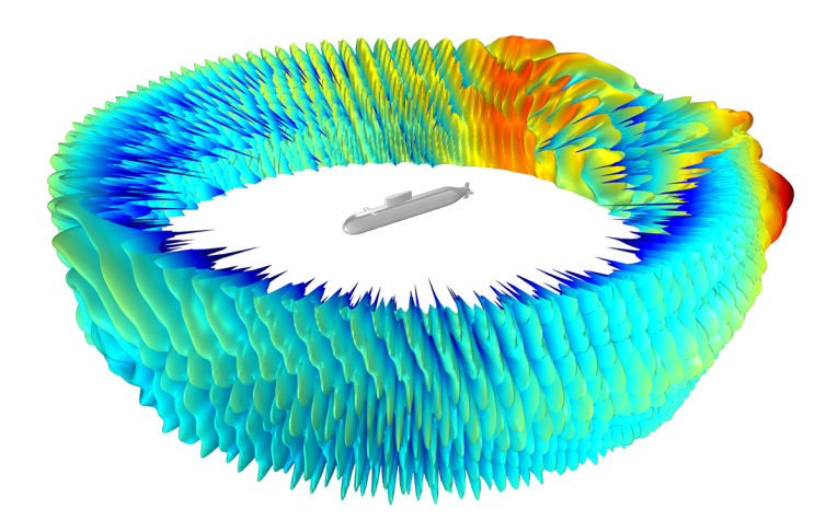
Certain classes of viscoelastic structural analysis are now more than 10 times faster. A new boundary element method formulation enables analyses of acoustics models that are up to an order of magnitude larger than previous versions. This type of analysis is useful within automotive and sonar research and development.
Clip planes enable easy selection of boundaries and domains inside of complex CAD models. Other graphics news includes visualizations that are partly opaque and partly transparent and the ability to make imported images part of a visualization. Material rendering of, for example, metals can be mixed with field visualizations and have environment reflections that look more real. Handling of larger CAD assemblies has improved with more robust solid operations and easier detection of gaps and overlaps in assemblies. In the Application Builder, new application templates provide a quick and intuitive way to create organized user interfaces for simulation apps.
The AC/DC Module includes an expanded material library with 322 new magnetic materials from Bomatec. The material data contains several types of permanent magnets, such as NdFeB, SmCo, and AlNiCo, with properties that depend on the temperature and the electromagnetic field. The new version of the AC/DC Module also provides specialized tools for the extraction of parasitic inductance with L-matrix computations, which is essential for designing printed circuit boards. New nonlinear material models are useful for modeling laminated iron core losses in electric motors and transformers.

The RF Module and Wave Optics Module provide a new option for port sweeps that enables faster computations of full S-parameter, transmission, and reflection coefficient matrices. For periodic structures within metamaterials and plasmonic devices, a new powerful polarization plot tool makes evaluation and visualization of transmitted and reflected waves significantly easier. The Ray Optics Module enables faster ray tracing and offers specialized tools for scattering from surfaces due to surface roughness and within volumetric domains due to Rayleigh and Mie scattering from particles.
Users can now simulate transient impact events in structural analyses using the mechanical contact functionality in the Structural Mechanics Module and MEMS Module. For users of the Structural Mechanics Module, contact analysis now includes functionality for analyzing mechanical wear with dynamic removal of material. The Structural Mechanics Module includes tools for crack modeling, providing J-integral and stress intensity factor computations as well as crack propagation based on a phase field method. Lower-dimensional elements can now be placed inside solids. Uses include the modeling of reinforcements for anchors, rebars, and wire meshes.
In the Composite Materials Module, the functionality for analyzing poroelastic effects has been expanded to include composite shells. Applications include the simulation of layered soil, paperboard, fiber-reinforced plastic, laminated plates, and sandwich panels.
The suite of nonlinear multiphysics material models in the MEMS Module now includes ferroelectric elasticity, which can be used for modeling nonlinear effects in piezoelectric materials such as hysteresis and polarization saturation. This functionality is also available by combining the AC/DC Module with either the Structural Mechanics Module or the Acoustics Module.
The CFD Module features new powerful tools for modeling combinations of separated and dispersed multiphase flow including support for compressible dispersed multiphase flow. In the Porous Media Flow Module and Heat Transfer Module, there is a new transport in porous media interface that enables users to model two-phase flow of moisture transport by vapor convection and diffusion coupled to liquid water convection and capillary flow. The Particle Tracing Module has new functionality for modeling droplet evaporation, which is important for understanding the spread of contagions as well as a range of industrial processes.
In the Heat Transfer Module, new functionality for surface-to-surface radiation lets users define surface properties that are sensitive to the direction of heat radiation, with applications such as passive cooling of solar panels. To model glass surfaces as exterior boundaries in radiation in participating media, the new semitransparent surface functionality lets you specify an external radiation intensity and account for the part of this incoming intensity that is diffusively or specularly transmitted through the surface.
The Corrosion Module now includes a material library with more than 270 instances of polarization data. The Chemical Reaction Engineering Module features a new tool for automatic reaction balancing with stoichiometric coefficient computations as well as three predefined thermodynamic systems for dry air, moist air, and water-steam mixtures, with a wide range of applications. There is also a new reactive pellet bed interface in the Chemical Reaction Engineering Module for multiscale modeling of fixed bed reactors by defining a microscale of very small pores inside the catalyst's particles and a macroscale of larger pores between the particles (bimodal pore structure).
Extensive New Features in Acoustics
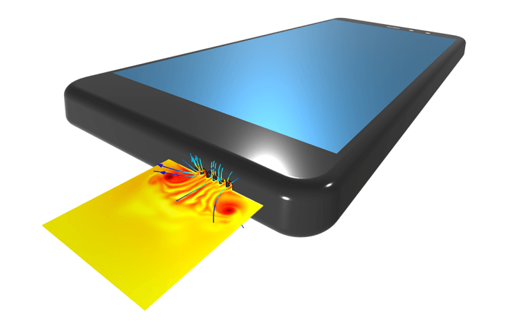
The updated COMSOL Multiphysics Acoustics Module can now be used to simulate high-intensity ultrasound as well as sound distortion in mobile device loudspeakers caused by nonlinear thermoviscous effects. New mechanical port conditions, available in the Structural Mechanics Module, Acoustics Module, and MEMS Module, simplify the analysis of vibration paths and mechanical feedback in applications involving the propagation of ultrasonic elastic waves, such as ultrasonic sensing and nondestructive evaluation.
Audio engineers will also appreciate the Acoustics Module's new room acoustics metrics for improving the sound quality of rooms and concert halls, including reverberation time and clarity based on ray acoustics simulations.
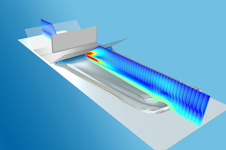
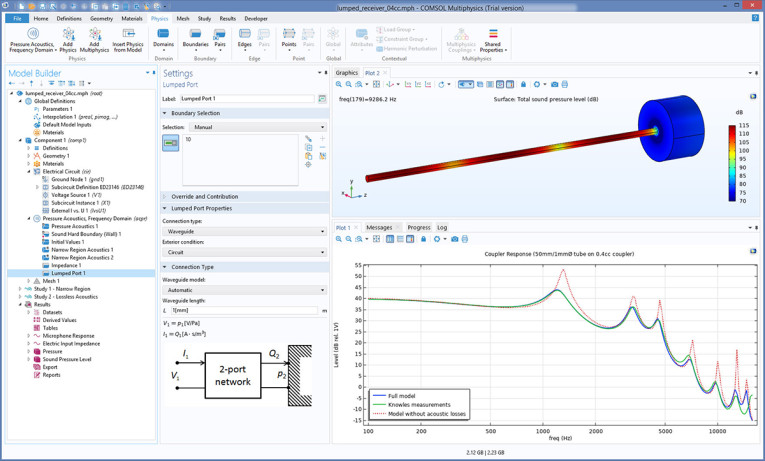
The new Lumped Port boundary condition in the Pressure Acoustics, Frequency Domain interface connects the end of a waveguide or duct inlet/outlet to an exterior system with a lumped representation. This can be an Electrical Circuit (with the AC/DC Module), a two-port network defined through a transfer matrix, or a lumped representation of a waveguide. Several representations and sources exist to describe the lumped system and to excite the system. When using the lumped port representation, it is assumed that only plane waves propagate in the acoustic waveguide. The condition simplifies, for example, setting up electroacoustic models where transducers or subsystems are described through a lumped equivalent model. This can be when modeling the miniature loudspeakers integrated into earbuds or hearing aids, or when modeling microphones and their inlet in smart speaker systems.
In the Pressure Acoustics, Boundary Elements interface, a new Excluded Boundary feature has been added. This can be used to exclude boundaries from the BEM model, which is particularly useful when using the Pressure Acoustics, Boundary Element interface in half-space or infinite baffle setups.
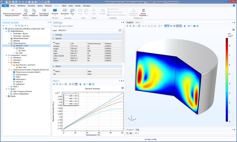
In high-fidelity and detailed absolute value acoustics simulations, it is necessary to know the material properties of moist air as a function of ambient pressure, ambient temperature, and relative humidity. Defining moist air is now possible using the predefined system for Moist Air in the Thermodynamics node. This functionality is available with the new Liquid & Gas Properties Module. One application is for the prediction of acoustic transfer impedance used in the procedure for reciprocity calibration of microphones.
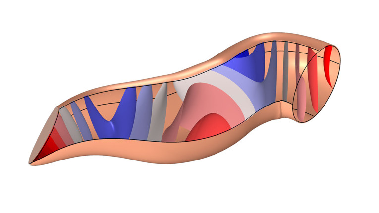
In the Pressure Acoustics, Frequency Domain interface, the new Thermoviscous Boundary Layer Impedance boundary condition adds losses due to thermal and viscous dissipation in the acoustic boundary layers at a wall. The condition is sometimes known simply as the BLI model. The losses are included in a locally homogenized manner, where they are integrated through the boundary layers analytically. The condition is applicable in cases where boundary layers are not overlapping. Formulated differently, it is not applicable in very narrow waveguides (with dimensions comparable to the boundary layer thickness) or on highly curved boundaries. Other than that, there are no restrictions on the shape of the geometry. The method is accurate when compared to the full thermoviscous formulation (if the conditions are met) and it is much less computationally intensive.
The Thermoviscous Boundary Layer Impedance boundary condition represents an engineering tool in pressure acoustics, comparable to the Narrow Region Acoustics feature. Applications are in the field of metamaterials, where the thermoviscous losses need to be included in an efficient manner to get physically correct results, but also in microacoustics in general, when modeling mobile devices, or measurement equipment.
The time explicit physics interfaces, which use the discontinuous Galerkin formulation (dG-FEM), benefit from a variety of performance improvements. There is a general speedup of up to 30% when solving 3D models with the Pressure Acoustics, Convected Wave Equation and the Elastic Waves, Time Explicit interfaces.
The time explicit interfaces can now be solved in combination with systems of ordinary differential equations (ODEs). This can, for example, be used to formulate user-defined frequency-dependent impedance boundary conditions in acoustics. The frequency dependency is approximated by an appropriate system of ODEs
The Elastic Waves, Time Explicit interface is now available as a 2D axisymmetric formulation. Additional post-processing variables have also been added to the Elastic Waves, Time Explicit interface including volumetric and deviatoric parts of the stress and strain variables, stress and strain invariants, and energy density and energy flow variables.
In the Ray Acoustics interface, rendering and computation time for impulse response have been greatly improved. The steps to set up impulse response are simpler and more consistent. Users can analyze and compute qualitative room acoustic metrics like clarity, definition, and reverberation time based on the computed impulse response. This is done using a new Energy Decay subfeature that can be added to an Impulse Response plot. In addition, users can export the computed impulse response signal to the waveform audio file format (.wav) for further analysis. The filter kernel functionality has been improved for impulse response computation, including user-specified definition of the filter kernel and visualization of the filters.
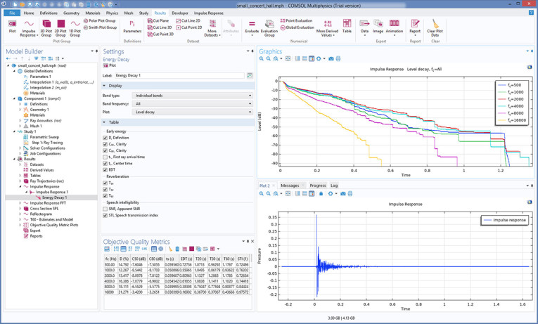
There are important improvements with respect to impulse response analysis, as well as new functionality, for the Energy Decay subfeature. This includes more precise computation of arrival time at the receiver when the source or the last reflection is close to the receiver. Direct sound now gets a consistent arrival time computation and summation of power. To get full advantage of the new functionality, models built in earlier versions need to be updated manually. The new qualitative room acoustic metrics, available when using the Energy Decay subfeature, are: reverberation times (T20, T30, and T60), clarity, definition, EDT, speech transmission index (STI), and the modulation transfer functions.
Users can now also export all 1D plots to .wav file format. This is particularly useful for acoustics results from a transient simulation or the impulse response in a ray acoustics simulation. Users can listen to the file or use it for further analysis in an external sound analysis tool.
When the Numeric (plane wave) option is used in the Port feature in a Thermoviscous Acoustics, Frequency Domain model, it now automatically detects the boundary conditions applied on the adjacent waveguide boundaries. The conditions are then automatically included when computing the mode shape of the propagating acoustic mode. This ensures physically consistent mode shapes for the port.
In pressure acoustics, a new option has been added to compute the mode shape and cutoff frequency for numeric modes in lossless systems. For a model without any losses, the new Computed lossless mode cutoff frequency option makes it possible to run a frequency sweep using a single Boundary Mode Analysis study for each port. The port features in Pressure Acoustics, Frequency Domain and Thermoviscous Acoustics, Frequency Domain now have the option to use power scaling for mode shapes. The default is to use amplitude scaling. With the power scaling option, the computed scattering parameters can be directly related to the power carried by a specific mode.
A new Three-parameter approximation JCAL model option has been added to the Poroacoustic feature in the Pressure Acoustics, Frequency Domain interface. The model is an approximation of the existing Johnson-Champoux-Allard-Lafarge (JCAL) model but only requires three porous parameters to be specified. The three parameters are the Porosity, the Median pore size, and the Standard deviation in pore size distribution. The model thus requires fewer inputs to define the porous matrix and the inputs in the model rely on averaged pore topology properties.
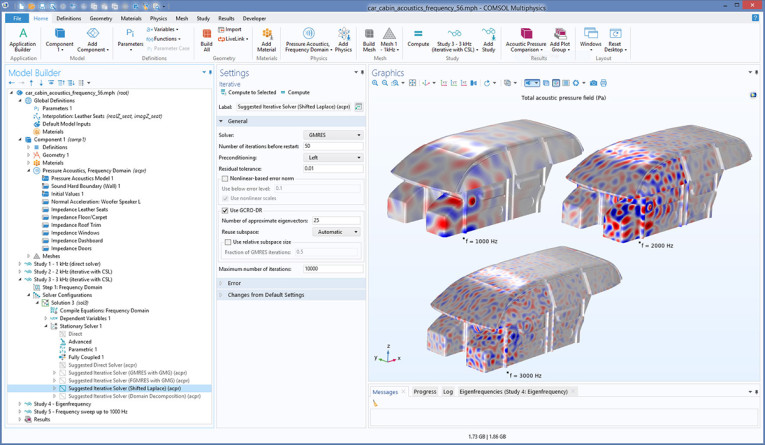
For pure Pressure Acoustics, Frequency Domain models, two new iterative solver suggestions have been added: one that uses the Shifted Laplace approach and another that uses Domain Decomposition. The iterative solver suggestions now automatically adds the necessary equation contributions on domains and at interior boundaries, between domains, to ensure solver efficiency. The Shifted Laplace solver is efficient for solving large models on a single machine with a lot of RAM while the Domain Decomposition method is suited for solving very large problems using distributed computation on a cluster.
New settings have been introduced in the Solid Mechanics interface that ensure a correct and efficient solver setup when solving elastic wave problems in the time domain. The settings are similar to the existing settings in the transient acoustics interfaces. In the Solid Mechanics interface node, a new Transient Solver Settings section has been introduced with an option to specify the Maximum frequency to resolve. This should be the maximum frequency content of the source's excitation or the maximum eigenmode frequency that can be excited. The automatically generated solver suggestion will have settings that use an appropriate solver method for wave propagation and ensure proper resolution in both time and space.
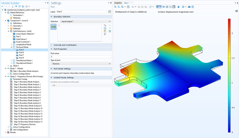
The new Port boundary condition, available with the Solid Mechanics interface, is designed to excite and absorb elastic waves that enter or leave solid waveguide structures. A given Port condition supports one specific propagating mode. Combining several Port conditions on the same boundary allows a consistent treatment of a mixture of propagating waves, for example, longitudinal, torsional, and transverse modes. The combined setup with several Port conditions provides a superior nonreflecting condition for waveguides to a perfectly matched layer (PML) configuration or the Low-Reflecting Boundary feature, for example. The port condition supports S-parameter (scattering parameter) calculation, but it can also be used as a source to just excite a system. The power of reflected and transmitted waves is available in post-processing.
When users initialize auxiliary dependent variables on particles, its possible to sample their initial values deterministically or, new with COMSOL Multiphysics version 5.6, randomly. When using the random option, users can sample from built-in normal, lognormal, or uniform distributions. For the Particle Tracing for Fluid Flow interface, users can also sample the initial particle mass or diameter from these distributions. When sampling the diameter, there is a built-in option to enter the Sauter mean diameter, a common way to describe the size distribution of aerosol particles. The Sauter mean diameter, along with other new variables for describing the particle size distribution, are also available in post-processing.
When rendering a Ray Trajectories plot, a new setting can be used to accurately render all intersection points of rays with surfaces in the geometry, even if they do not correspond to output time steps in the solution data. To perfectly render every intersection point of every ray with a surface, the old implementations scaled quadratically with the number of rays, whereas the new behavior scales linearly with the number of rays, potentially giving a massive speedup when the number of rays is very large. This also applies to the calculation of intersection points between rays and a sphere, hemisphere, or plane.
Full details on the Acoustics Module updates and direct links to tutorials are now available online here.
COMSOL Multiphysics 5.6 is available now. COMSOL Multiphysics, COMSOL Server, and COMSOL Compiler software products are supported on Windows, Linux, and macOS. The Application Builder tool is supported in the Windows operating system.
www.comsol.com