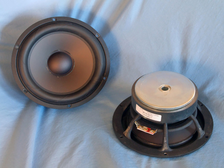
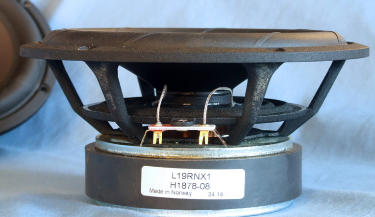
The Titan line, which began with the 27TAC/GB 1” dome tweeter and the L16RNX3 5.25” woofer, all feature FEA-optimized motor systems, copper caps and shorting rings, and titanium voice coil formers in combination with matte black aluminum cones. Features for the new L19RNX1 include a proprietary injection-molded aluminum frame with six narrow spokes to minimize reflections back into the cone (see Photo 2), a lightweight curved-profile matte black aluminum cone, a copper tube shorting ring (Faraday shield), a FEA-optimized motor structure with a 39 mm (1.5”) diameter non magnetically conductive titanium voice coil former wound with round copper wire, a fairly substantial 200 W short-term power handling capacity, and gold-plated terminals. Note that the outside perimeter of the aluminum cone is turned down to increase stiffness at the edge point where the surround is attached.
Compliance is provided by a radial reinforced NBR surround that reduces surround resonances and prevents surround breakup at high excursion and works in conjunction with a black flat 4” diameter spider (damper). For cooling, the frame is completely open beneath the spider mounting shelf, and with a small 12 mm diameter pole vent, substantial air can be pumped past the voice coil and over the front plate.
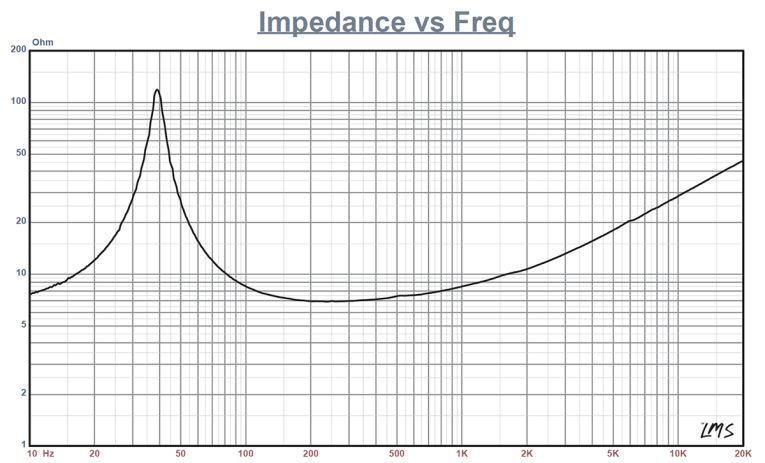
I began characterizing the L19RNX1 using the LinearX LMS analyzer and VIBox to create both voltage and admittance (current) curves with the driver clamped to a rigid test fixture in free-air at 0.3V, 1V, 3V, 6V, 10V, and 15V. The 15V curve was more than linear enough to obtain a good curve fit, which is unusual for a 6.5" driver and is certainly due to the larger surround incorporated into this device.
Following my established protocol for Test Bench testing, I no longer use an added mass measurement (for Vas calculation) and instead use the physically measured Mmd supplied by the manufacturer. I post-processed the 12 550-point sine wave sweeps for each L19RNX1 sample and divided the voltage curves by the current curves to generate impedance curves, with the phase derived using the LMS calculation method. Then I imported the collected data, along with the accompanying voltage curves into the LEAP 5 Enclosure Shop software.
Because Thiele-Small (T-S) data provided by the majority of OEM manufacturers is generated using either the standard model or the LEAP 4 TSL model, I additionally created a LEAP 4 TSL parameter set using the 1 V free-air curves. I selected the complete data set, the multiple voltage impedance curves for the LTD model, and the 1 V impedance curve for the TSL model in the transducer parameter derivation menu in LEAP 5 and created the parameters for the computer box simulations.
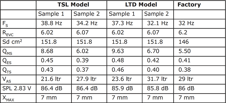
Figure 1 shows the 1 V free-air impedance curve. Table 1 compares the LEAP 5 LTD and TSL data and factory parameters for both of SEAS L19RNX1 samples. LEAP parameter calculation results correlated reasonably well with the SEAS factory published data. SEAS does use a somewhat more conservative Sd number, but the effect appears relatively minor here.
I followed my established protocol and proceeded setting up computer enclosure simulations using the LEAP LTD parameters for Sample 1. I programmed two computer box simulations into LEAP 5—the first one a Butterworth sealed box with a 0.44 ft3 volume with 50% fiberglass damping material; and the second simulation a Quasi Third-Order Butterworth (QB3) vented enclosure alignment with a 0.75 ft3 volume (15% fill material) tuned to 33 Hz.
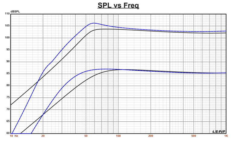
Figure 2 displays the results for the SEAS L19RNX1 in the two enclosures at 2.83 V and at a voltage level sufficiently high enough to increase cone excursion to Xmax + 15% (8 mm for the L19RNX1). The sealed box alignment had a F3 = 56 Hz (F6 = 44 Hz) with a Qtc=0.68, while the QB3 alignment produced a 3 dB down frequency of 40 Hz (F6 = 33 Hz).
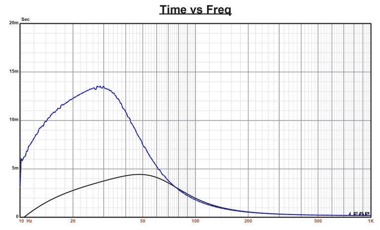
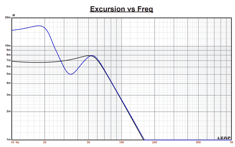
Increasing the voltage input to the simulations until the maximum linear cone excursion criteria was reached resulted in 104 dB at 22.5 V for the smaller sealed box simulation and the 106 dB at 25 V input level for the larger vented enclosure. Figure 3 shows the 2.83 V group delay curves. Figure 4 shows the 22.5 V/25 V excursion curves.
In the case of the QB3 vented box simulation, excursion goes beyond the Xmax + 15% number at frequencies lower than about 26 Hz, so a 20 Hz steep (24 dB/octave) high-pass filter would be a useful addition and could prevent over excursion and distortion.
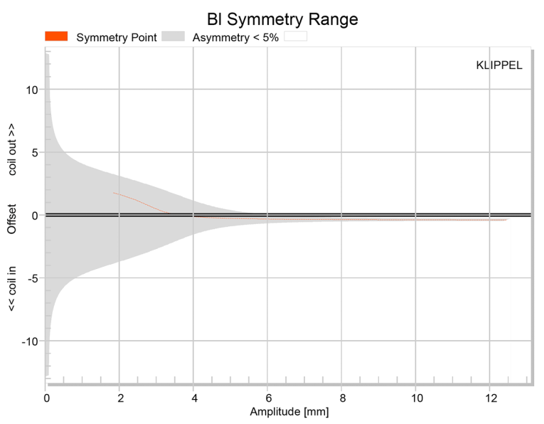
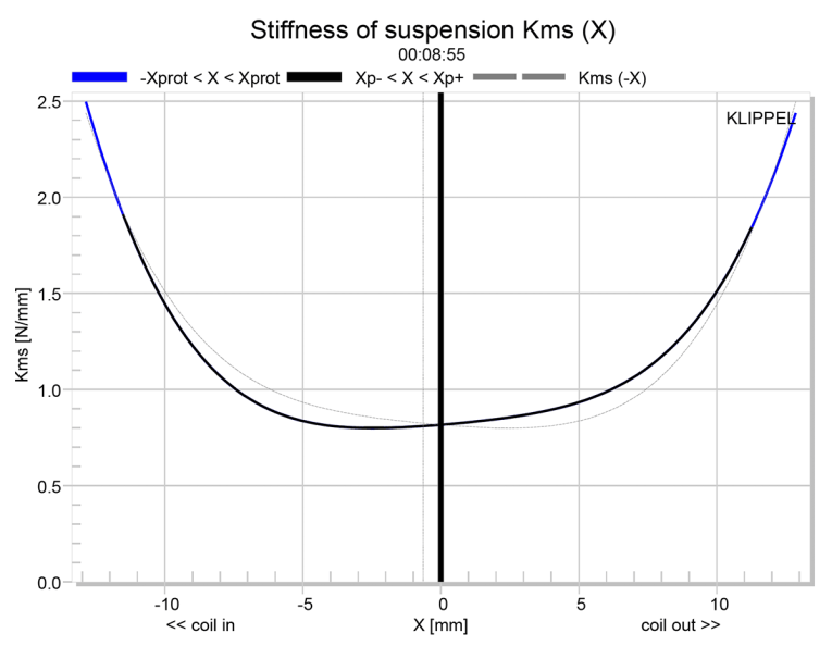
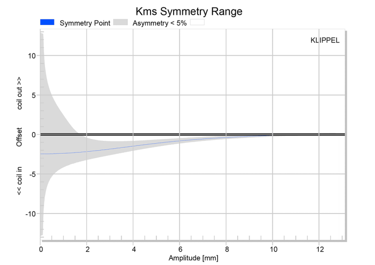
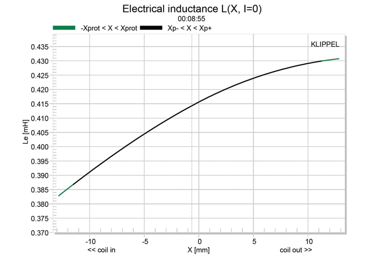
Figure 7 and Figure 8 show the Kms(X) and Kms symmetry range curves for the SEAS L19RNX1. The Kms(X) curve shown in Figure 7 is somewhat asymmetrical in both directions and tilted toward the coil-out direction, as well as having small amount of coil-in offset. Looking at the Kms symmetry range plot shown in Figure 8, there is a coil-in displacement of 1.5 mm at 4 mm, but this diminishes to 0.32 mm at the physical Xmax 7 mm coil position. Displacement limiting numbers calculated by the Klippel analyzer for the SEAS L19RNX1 were XBl at 82% Bl = 6.9 mm and for XC at 75% Cms minimum was 7.2 mm, which means that for the L19RNX1, the Bl is the slightly more limiting factor for prescribed distortion level of 10%. However, both numbers were right at the driver’s physical Xmax, so this is nicely balanced.
Figure 9 gives the inductance curves L(X) for the SEAS L19RNX1. Inductance will typically increase in the rear direction from the zero rest position as the voice coil covers more pole area, however because of the copper tube shorting ring, inductance decreases in the rear (coil-in) position. From Xmax out to Xmax in, the inductance range only varies by 0.02 mH, which is really excellent inductive performance.
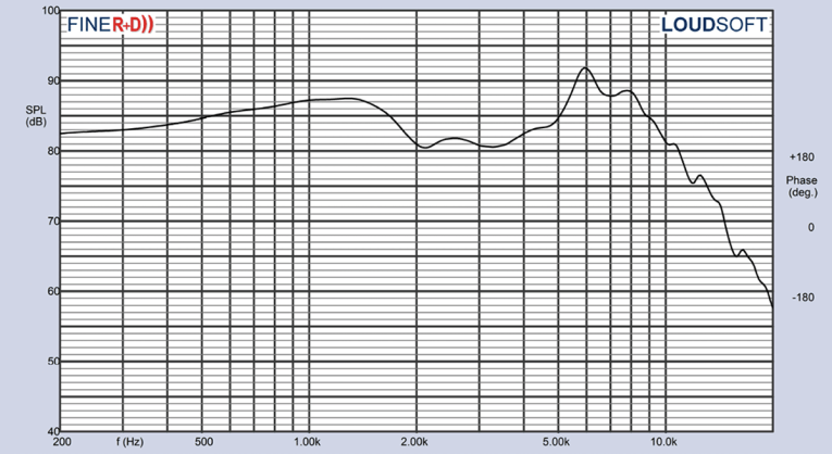
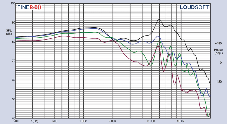


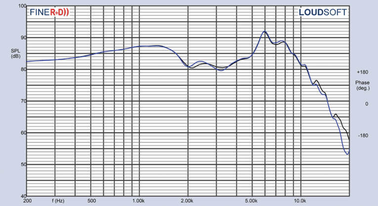
Figure 10 shows the SEAS L19RNX1 on-axis response indicating a rather smooth rising response to about 1.5 kHz and then a declining response that is -6 dB at 1.8 kHz relative to 1.5 kHz, with the aluminum break-up mode starting at about 6.0 kHz, where the driver begins its low-pass roll-off. Figure 11 displays the on- and off-axis frequency response at 0°, 15°, 30°, and 45°, showing somewhat more directivity than most home audio 6.5” woofers. The -3 dB at 30° with respect to the on-axis curve occurs at 1.45 kHz, so a cross point in that vicinity should work well to achieve a good power response. This could be done in a three-way configuration with a dome midrange and dome tweeter, or in a two-way configuration with a larger air motion transformer (AMT) or ribbon device capable of being crossed that low.
Figure 12 gives the normalized version of Figure 11, while Figure 13 displays the CLIO horizontal polar plot (in 10° increments) for the SEAS L19RNX1. And finally, Figure 14 gives the two-sample SPL comparisons for the L19RNX1, showing a close match (less than 0.5 dB) throughout the operating range up to 2 kHz.
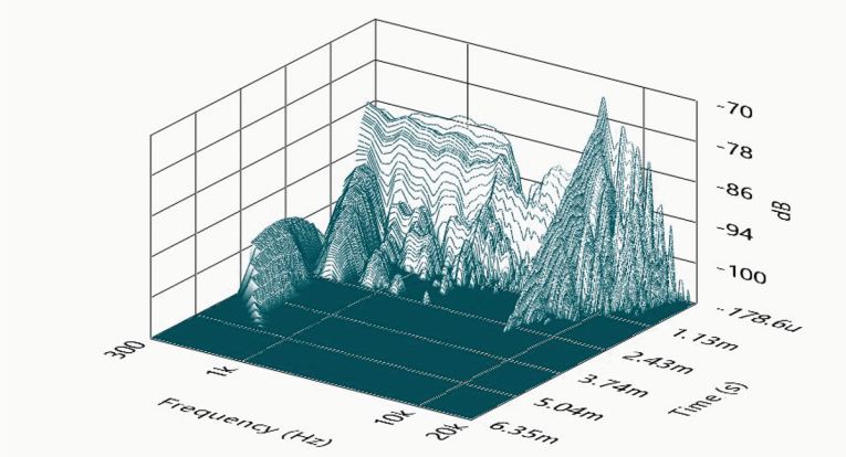
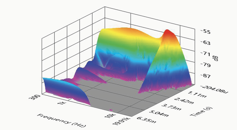
I then employed the SoundCheck 17 software to get the 2.83V/1m impulse response and imported the data into Listen’s SoundMap Time/Frequency software. Figure 16 shows the resulting cumulative spectral decay (CSD) waterfall plot. Figure 17 shows the Wigner-Ville plot (used for its better low-frequency performance). Looking at all the data I collected for the new 19 series aluminum cone SEAS L19RNX1, this is a high power handling and high output driver for a 6.5”, which I believe was the goal of the 19 series. This driver portrays the kind of engineering integrity and high build quality you would expect from this iconic Norwegian high-end OEM driver manufacturer.
From its founding in 1950 as a spin-off of the Norwegian radio manufacturers Radionette and Tandberg, SEAS has been dedicated to creating loudspeakers with superior sound reproduction. The company, whose name means Scandinavian Electro Acoustic Systems, has remained in the forefront of European driver manufacturing for more than 70 years. For more information, visit www.seas.no. VC
This article was originally published in Voice Coil, July 2020.