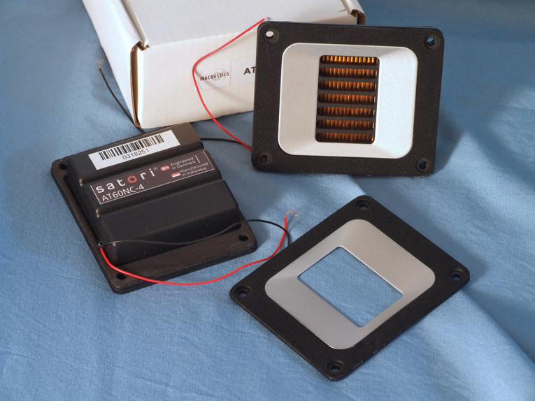
Features for the Satori AT60CN-4, designed in Denmark by Danesian Audio, include a damped foil and Kapton 43mm × 29mm pleated AMT diaphragm, an optimized rear chamber, two-part faceplate, 91dB sensitivity, and a diaphragm area (Sd) of 12.6 cm2, just somewhat smaller area than a 30mm dome tweeter.
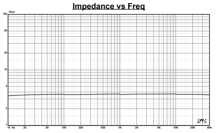
Testing commenced using the LinearX LMS analyzer to produce the 300-point stepped sine wave impedance plot shown in Figure 1. With a nominal 4Ω impedance, the AT60CN-4 has a 3.78Ω DCR, with minimum impedance of 3.67Ω and at 2.64kHz. While the factory specification of the Fs resonance of the driver is 2200Hz, as can be seen, there is no discernible resonance to AMT transducers.
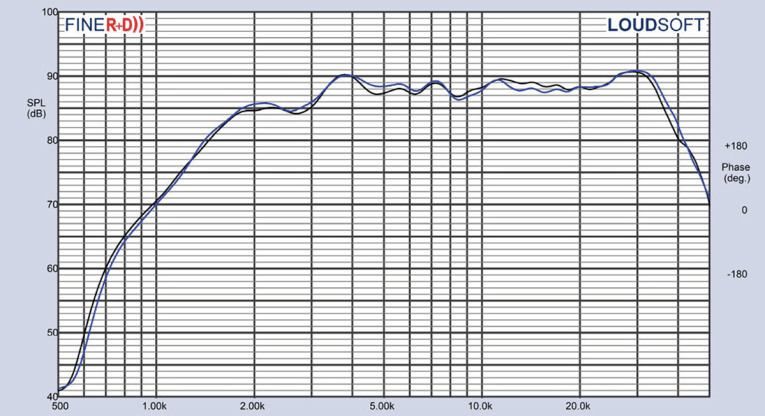
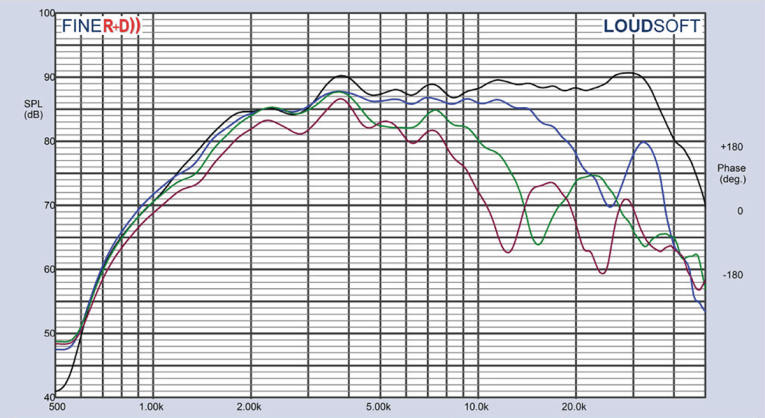
For the next set of SPL measurements, I surface-mounted the AT60CN-4 AMT combination with an enclosure that had a 10” × 5.5” baffle and measured both the horizontal and vertical on- and off-axis at 2V/0.5m (normalized to 2.83V/1m) from 0° on-axis to 45° off-axis using the LoudSoft FINE R+D analyzer and the GRAS 46BE microphone (supplied courtesy of LoudSoft and GRAS Sound & Vibration). Due their asymmetrical shape, AMTs have a vertical directivity that is significant enough to be taken into account, which is why I performed a series of vertical plane measurements.
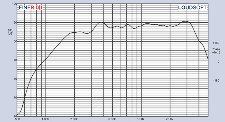
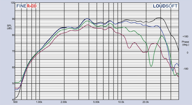
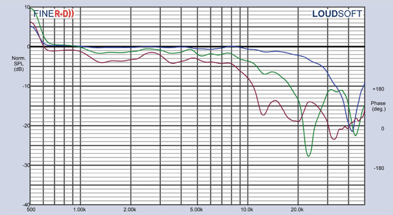
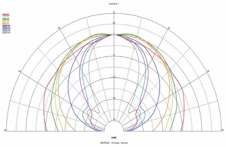
Figure 2 shows the AT60CN-4’s on-axis frequency response, which is ±1.5dB with no major anomalies from 3.2kHz to about 26kHz, beginning its second-order low-pass roll-off at 30kHz. Figure 3 shows the 0° to 45° on- and off-axis response in the horizontal plane. Figure 4 shows the normalized horizontal plane response. While Figure 5 shows the 180° horizontal polar plot (in 10° increments with1/3 octave smoothing applied) that was generated by the CLIO Pocket analyzer and accompanying microphone (courtesy of Audiomatica SRL).
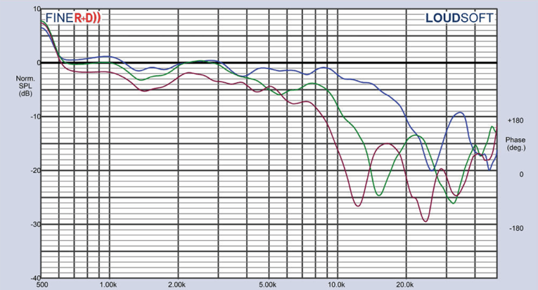
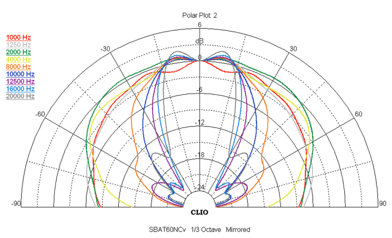
For the vertical plane of the AT60CN-4, Figure 6 gives the 0° to 45° response, normalized in Figure 7. Figure 8 shows the CLIO Pocket analyzer-generated power plot. Last, Figure 9 displays the two-sample SPL comparison, showing the two SB Acoustics Satori AT60CN-4 driver samples to be matched within 1.5dB or less throughout the entire operating range of the transducer.
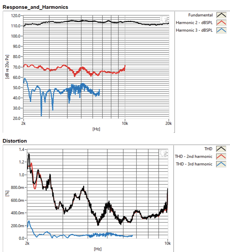
For the remaining series of tests, I again set up the Listen AudioConnect analyzer and 1/4” SCM microphone (provided to Voice Coil by Listen, Inc.) to measure distortion and generate time-frequency plots. For the distortion measurement, I mounted the AT60CN-4 in the same enclosure as was used for the frequency response measurements, and set the SPL to 94dB at 1m (5.40V determined by using a pink noise stimulus generator and internal SLM in the SoundCheck V18 software). Then, I measured the distortion with the Listen microphone placed 10cm from the mouth of the AMT diaphragm. This produced the distortion curves shown in Figure 10. Note the extremely low third-harmonic level.
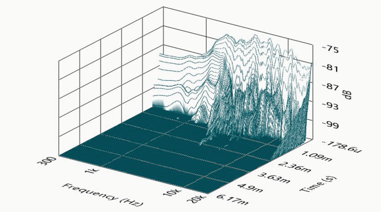
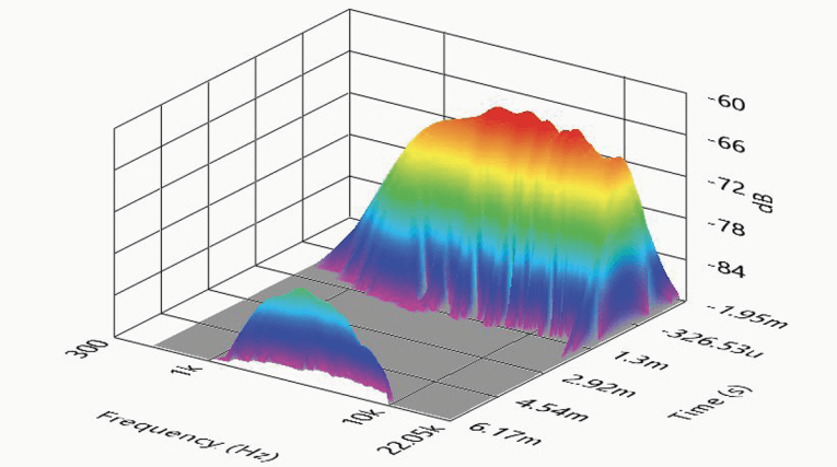
Following this test sequence, I then set up SoundCheck to generate a 2.83V/1m impulse response curve for this AMT transducer and imported the data into Listen’s SoundMap Time/Frequency software. Figure 11 shows the resulting cumulative spectral decay (CSD) waterfall plot. Figure 12 shows the Short Time Fourier Transform (STFT) plot. Looking over all the data, the Danesian-designed AMT definitely exhibits very good performance. For more information, visit www.sbacoustics.com. VC
This article was originally published in Voice Coil, March 2021.