 In this article series, we are examining ways to create a low-cost system for lab-grade audio electronics measurements. To this point, I’ve looked at the hardware and software bits of the sound-card based measurement system. The last remaining piece is the user.
One of the hazards of computer-based measurement systems is their uncanny ability to acquire impressive amounts of bad data in a surprisingly short time. The only way to minimize this is by understanding the measurement, choosing the right measurement parameters, and recognizing the artifacts in the data that are due to the parameter choices. Unfortunately, this is the hardest part of the process and unavoidably requires some understanding of the math.
I’ll try to make this as painless as possible and make clear what the results of the math mean, rather than going through the derivations with the utmost of rigor. The power of the computer lets us freely use mathematical transforms, which are powerful tools if understood and correctly used. The most basic and frequently used one is the Fourier Transform (FT).
Fourier Transform: Threat or Menace?
Signals can be characterized in two ways: amplitude (usually voltage) vs. time or amplitude vs. frequency. The FT is a mathematical means of converting from one view to the other. For a continuous function of time a(t), the Fourier Transform F(f) is defined as:

where a(t) is the signal in the time domain. Note that the integral is over an infinite amount of time and the signals are assumed continuous (we’ll come back to this shortly).
The math aside, it is important to understand that the time and the frequency views are exactly equivalent. All the same information is contained in them and they may be interconverted at will. The choice of frequency or time domain is arbitrary and will depend on what’s more convenient for the particular phenomenon you’re testing.
For example, if I wanted to examine an amplifier’s stability, I might run a square wave test and, in the time domain, look for overshoot on leading and trailing edges or even ringing on the top of the waveform. There would be no particular reason to convert the signal to the frequency domain for analysis, even though I could get the same information.
On the other hand, if I wanted to understand an amplifier’s distortion characteristics, I could apply sine waves of different frequencies and levels, then squint at the sine waves on the amplifier’s output and try to see if they looked different. The problem is that eyeballing the results on an oscilloscope screen does not give much sensitivity: distortion has to be pretty gross to be visible. It’s also not very quantitative. And to compound the difficulties, the type of distortion will not be clearly evident (although the symmetry between the top and the bottom of the sine wave will give some indication of whether the predominant distortion is even or odd order).
A much better way to quantify and characterize the distortion is by taking the amplifier output and transforming it into the frequency domain, creating a frequency spectrum. The basic Fourier theorem that we learn in freshman math is that any periodic signal, irrespective of its shape, may be broken down into a fundamental sine wave frequency and harmonics (that is, sine waves with frequencies that are whole number multiples of the fundamental frequency); the relative magnitudes and phases of the harmonics determine the waveform’s shape in the time domain.
So the frequency spectrum will be convenient for quantifying the linearity, showing what new frequency components (harmonics) are present in the output signal that weren’t present in the input signal and what their relative sizes are, which is the basic definition of distortion. An undistorted sine wave will have only one frequency component, the fundamental frequency.
Distortion adds new components at the harmonics. The old-fashioned way of determining the frequency spectrum was with a wave analyzer. Essentially, a wave analyzer is a narrow tunable bandpass filter attached to an AC voltmeter. A signal is fed to the input of the device under test (DUT).
The DUT’s output is connected to the tunable filter’s input, and the filter’s frequency is swept. The AC voltmeter records the output voltage as a function of frequency. As it sweeps through the harmonic frequencies, a spectrum can be recorded. The most popular high-quality wave analyzer was the Hewlett-Packard 3581A, which, although expensive in its day, can be found online for remarkably low prices. It’s slow, inconvenient, and not terribly sensitive, but it’s my back-up instrument that I use to check my work when readings I get with a sound card look funny.
With the advent of electronic computing power, FT methods became a better solution. In particular, the Fast Fourier Transform (FFT) was an efficient algorithm for computing the FT of a sampled waveform in a finite time window. [It should be noted that we’ve silently slid from a Fourier transform (continuous function) to a Discrete Fourier Transform (set of sampled points); that’s a bit beyond the scope of this article, but I can hear engineers and mathematicians wincing.]
In a basic FT measurement, a waveform is sampled in the time domain (just like the digital recording of music) and the time domain record for the length of the measurement (called a frame) is Fourier-transformed using an FFT to give a frequency spectrum. That’s the simple view—the reality starts getting a bit more complicated.
Just as in digital recording, we sample a signal at time intervals tS. Equivalently, we can say that we sample at a frequency of fS = 1/ tS (sample rate). The numbers corresponding to each sample (time point and measured amplitude at that time) can be stored in the computer memory or in a file as a data record.
The number of data points in the data record is equal to the sample rate multiplied by the measurement time (which is ideally infinite, but is generally limited to a finite interval). For example, if the sample rate is 48 kHz and we sample for 0.5 seconds, the data record (which we will call a “frame”) will contain 24,000 points. For most software, one selects the number of data points in each frame, from which you can calculate the measurement time:
Measurement Time per frame = number of data points/sample rate.
The FT of that time record of the samples will contain half the frame’s number of time/amplitude data points (remember that the frequency range is Nyquist limited to half the sample rate), so we can calculate the distance between the FT’s frequency/amplitude points (and frequency resolution) from:
Frequency Resolution = 2x frequency range/number of data points = sample rate/number of data points.
What are the implications of these basic relationships?
Although we draw the frequency spectrum as a continuous line, in reality, each frequency is not actually a point, but rather an interval of frequencies with a width equal to the resolution. It is referred to as a “bin,” largely because all amplitude components within that interval are essentially grouped together as a package. You can think of a bin as a narrow band-pass filter. As the number of samples in a frame increase (for a given frame length in time), the width of the bins narrow. In the limit of an infinite number of points in a frame, the bins shrink to points, resolution becomes infinitely fine, and the frequency spectrum is continuous.
If the sampled signal is a pure sine wave, the FT of the data record ideally will be a single spike at the fundamental. If we distort the sine wave a bit, other spikes at whole-number multiples of the fundamental frequency appear, as expected. The spikes at frequencies that are even whole-number multiples of the fundamental are called (logically) even-order harmonics, and analogously, the harmonics appearing at odd-number multiples are called odd-order harmonics.
Some rules of thumb for relating frequency and time domain:
• Odd-order distortion components cause symmetrical distortion around the horizontal (time) axis in the time domain. So, for example, if you see a flattening of both the tops and the bottoms of a sine wave, you know that the frequency spectrum will be dominated by odd order harmonics. The extreme example is a square wave, which contains all possible odd order harmonics and no even-order ones.
• Even-order distortion components cause non-symmetrical distortion around the time axis. So, for example, if you see flattening of the tops of a sine wave but not the bottom, the frequency spectrum is dominated by even-order harmonics.
• “Sharper” features in a waveform (e.g., the leading and trailing edges of square waves or the small zero-crossing notch from crossover distortion) are indicative of high-order harmonics (i.e., where the whole number multiples are large).
Windows (Not the Microsoft Kind)
A real waveform and its set of samples is not infinite in length. It will have a start and a stop. The longer the sampling window, the lower the frequency that can be measured. This makes intuitive sense if you consider that you want at least one full cycle of the lowest frequency of interest to fit within the sampling time. So for a 10-Hz wave, you want a sampling window that is at least 0.1 seconds long.
Let’s say that we have a sample rate of 48 kHz. Then, the minimum frame to measure 10 Hz would be 4,800 data points. The number of data points also sets the measurement resolution. In this example, each frequency point will be 10 Hz from its neighbor, so that one will not be able to resolve a frequency more precisely than that.
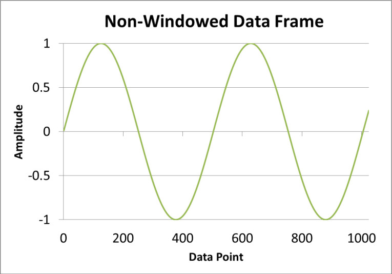
You’ll often hear the objection, “Fourier transforms are only good for periodic or repetitive signals.” In a formal sense, since the FT works on periodic signals, the finite length of the frame conceptually represents the period. Then, the periodic signal (in a mathematical sense) is an infinite string of the frames. This brings up another complication — continuity. The waveform’s values at the point where the conceptual frames join up have to be equal or the resulting spectrum will be misleading because of a discontinuity where the waveforms meet.
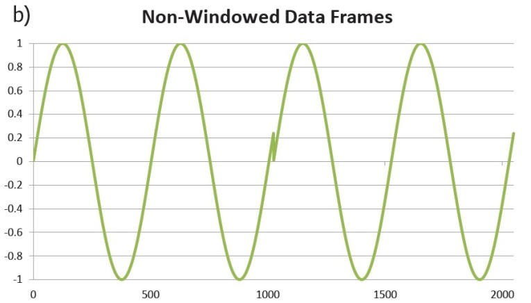
To illustrate, if the measured signal is a sine wave, it’s unlikely that its period will be such that its zero crossings end up perfectly at the start and stop of the frame. It’s far more likely that the frame edges will correspond to some other point on the waveform (see Figure 1a). When we conceptually join the frames to make a periodic signal (with the period being the time span of the frame), the discontinuities where the frames meet up are evident (see Figure 1b). These discontinuities are a function of the finite sampling window and aren’t part of the actual waveform we want to analyze.
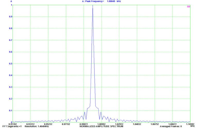
What’s the effect of this discontinuity? In the unlikely event that the sine wave is at a zero crossing at the beginning and end of the frame, the discontinuity disappears. In the far more likely event that the signal will have some non-zero value at the edges of the frame, the frequency domain spectrum obtained from the FT will no longer be a single line at the sine wave frequency. Instead, it will be broadened from the spectrum “leaking” into adjacent bins (see Figure 2), which smears out the spectrum. Note that the vertical axis in Figure 2 is linear, so the “wings” on either side of the fundamental frequency are only 20 dB down. The apparent noise floor will also be significantly higher from that same leakage. Clearly, this is not desirable for precision measurement!
To overcome this problem, we use a trick called “windowing” or “apodization.” Ideally, the sampled signal would be zero at the frame edge, so we can multiply it by a function that is in fact zero on each edge of the frame, but unity in the center of the frame. Generally, the variation from edge to center is smooth and continuous. Most common window functions look more or less Gaussian to the eye (though they are not at all the same mathematically).
Since we’re now putting a new function (the window) into the signal data record, there will be both good and bad effects on the calculated spectrum, and to maximize the good and minimize the bad, there are a variety of possible window functions. The tradeoffs are between side-lobe suppression, frequency resolution, and amplitude accuracy. Therefore, the specific choice of window function will depend on what it is you’re trying to measure. I have compiled a non-comprehensive survey of some common window functions.
Rectangular: This is actually no window at all, and we’ve seen the effect on a sine wave spectrum. Sometimes a rectangular function does have its uses. It is likely the window of choice if you’re looking at a frame containing a single transient event, since we do not want the calculation to vary depending on where in the frame the transient is sampled. Likewise, it’s the window of choice for measurement of random noise.
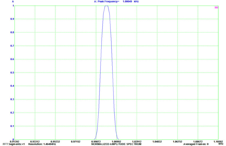
Flat-Top: Despite its name, the flat-top does not have a flat top. Sharp peaks in the frequency domain show flattened tops with this window, thus the name. It is derived from a sum of cosines:

where N is the number of samples in the frame. An FT of a sine wave using the flat-top window is shown in Figure 3. A flat-top window is a good choice if you’re trying to accurately measure the amplitude of a frequency component. It is a poor choice if you’re trying to resolve two closely spaced (in the frequency domain) signals, since it broadens the spectral lines.
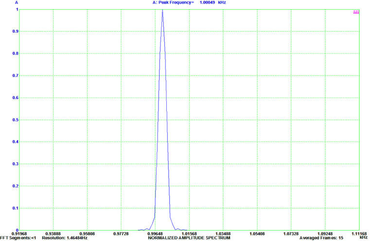
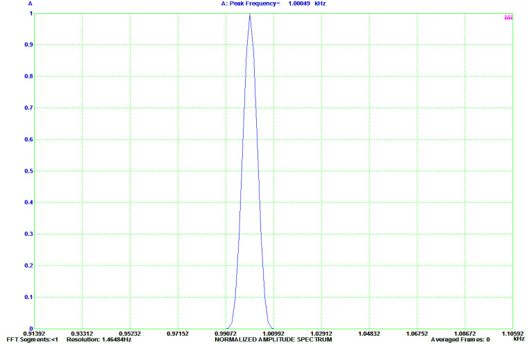
Hanning: The Hanning is a good general purpose window, defined by the rather simple function:

It does not have the amplitude accuracy of a flattop, but can resolve closely spaced signals of similar amplitude. Figure 4 shows an FT of a sine wave using a Hanning window. The Hanning should not be confused with the Hamming, which is similar window, but not the same.
Blackman-Harris: The Blackman-Harris window is defined by:

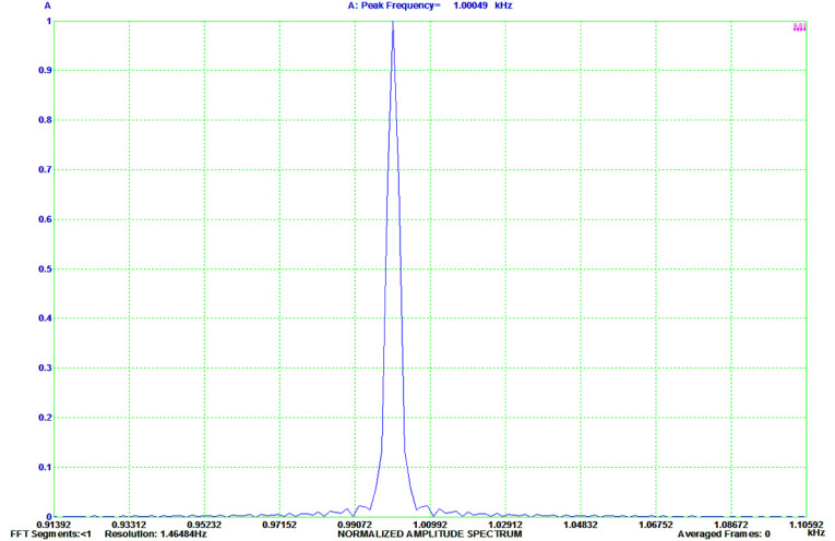
It has better amplitude accuracy than the Hanning, but not as good as the flat-top. It’s most useful for resolving two closely spaced signals of different amplitude (e.g., power supply intermodulation sidebands near the fundamental) because of its superior side-lobe suppression. Figure 5 shows an FT of a sine wave using a Blackman-Harris window.
Kaiser: The Kaiser window is derived from Bessel functions, rather than cosines, and is defined by:

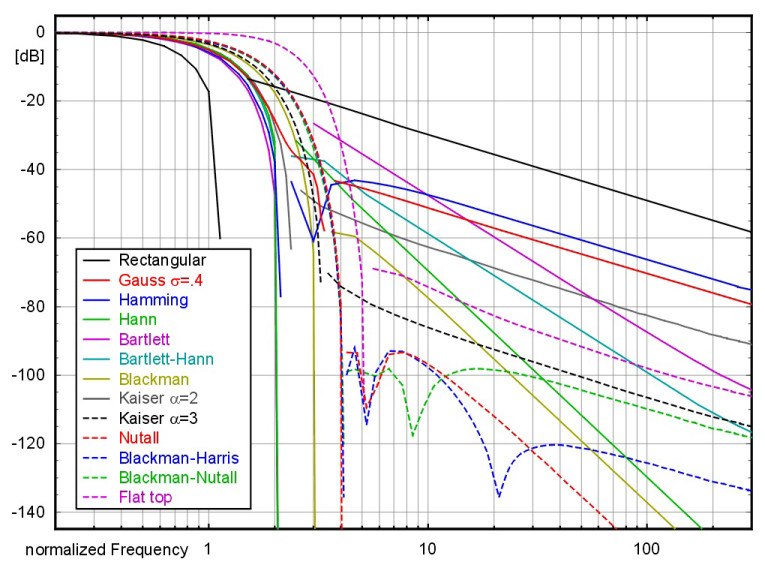
where IO is the zero-order Bessel function of the first kind and α is a constant that determines the overall shape of the window. The Kaiser window is most often used for high dynamic range signals where it offers a good trade-off between amplitude accuracy and peak width to resolve small signals close in frequency to large ones (much like Blackman-Harris). Figure 6 shows an FT of a sine wave using a Kaiser window. Figure 7 shows a comparison of various window functions and their effect on a single spectral line.
(Image courtesy of Marcel Mueller, used under Creative Commons license)
Note that all the window functions are defined as being equal to zero outside of the frame. Most of the software packages I mentioned have selectable window functions (the Virtins enables you to create your own and add them to its already-huge list). It’s worth experimenting with them using known input signals to get an intuitive feel for their characteristics.
Averaging
A way to increase the signal-to-noise ratio (SNR) in an FT measurement is to take the average of multiple frames. The signal increases by 6 dB with each average because it’s correlated between frames, but the noise increases by 3 dB because it is uncorrelated (that’s why it’s noise!). Another way to say this is that the correlated signal adds as voltage but the uncorrelated noise adds as power. So for each doubling in the number of frames in the average, the signal-to-noise improves by 3 dB.
In general, one of the DUT’s attributes is its noise, and we want to measure it rather than average it out, but we do want to reduce the fluctuations between frames (i.e., the noise intrinsic to the measurement). In measurement parlance, the distinction between the fluctuations in the measurement and the DUT’s noise is referred to as detector noise and source noise, respectively. The way detector noise is handled in the calculations, rather than taking the vector sum of the frames’ data, is to average the frames via a root-mean-square sum. That averages out the measurement deviations from the DUT’s noise floor (but not the DUT’s noise) by treating any deviation as positive and uncorrelated with the deviations in other frames.
In summary, increasing the number of averaged frames reduces the random fluctuation in the measurement compared to non-random signal by √N, where N is the number of averaged frames. Measurement time is increased in direct proportion to N, of course.
Wrap Up
In the next installment, I will run some example measurements that bring together the various ideas discussed in this series, and show how they are interpreted. You’ll get a sense of how to use these remarkably powerful and accessible tools. ax
This article was originally published in audioXpress, October 2015.
Resource
F. J. Harris, “On the Use of Windows for Harmonic Analysis with Discrete Fourier Transform,” Proceedings of The Institute of Electrical and Electronics Engineers (IEEE), January 1978.
 About the Author
Stuart Yaniger has been designing and building audio equipment for nearly half a century, and currently works as a technical director for a large industrial company. His professional research interests have spanned theoretical physics, electronics, chemistry, spectroscopy, aerospace, biology, and sensory science. One day, he will figure out what he would like to be when he grows up.


