Soldering today is even more difficult with the effort underway to remove hazardous materials from the environment. Much solder used today is lead-free. I decided to test the different types of solder to see which one works and sounds best to me.
Yellow Speaker
There seems to be controversy over what testing means in audio. Measuring a difference does not mean you can hear it. For example, if you paint your loudspeakers yellow, it would be a great surprise to hear a difference in a blind test. You could certainly measure and document the change in color. If you asked a panel of listeners to indicate their preferences, there would probably be a significant difference of opinion about the sound quality if they were looking at the loudspeakers.
I personally would ignore this data. Even with identical components, there are differences. The evidence that color changes sound quality would need to be almost overwhelming before it would even be worth considering. On the other hand, if my ears tell me there is a difference between two audio chains and I cannot measure it, that does not mean it is not there. The color change in the previous example probably is the wrong method to determine audio differences. I could measure frequency response, distortion, or other parameters to find the difference. Even if all the measurements were exactly the same, but my ears told me there was a difference, then it would be a question as to where my measurements failed or whether there was something else that should be measured.
Test Setup
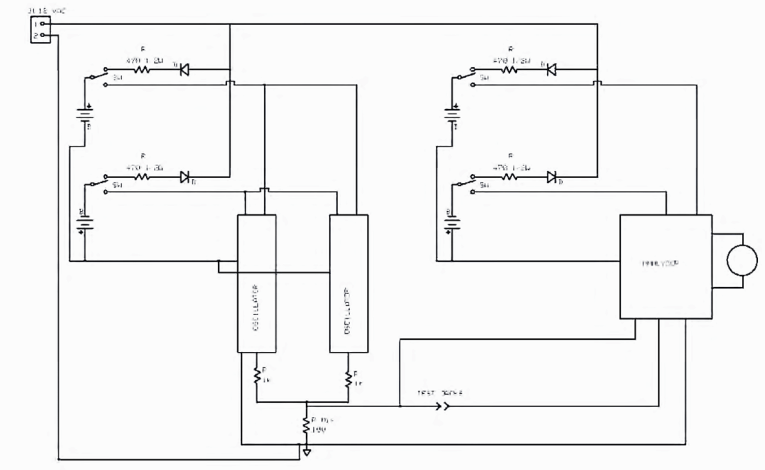
Starting with a simple experiment seemed the way to proceed with investigating solder. I used a setup with two lead-free printed circuit boards and two matching paths, pads connected by 54 jumpers. The jumpers were made from the cutoff tinned copper leads of lead-free precision resistors. Low temperature coefficient resistors also have low coefficient leads!
I soldered one set of jumpers with Kester .031″ 62% tin 36% lead and 2% silver rosin core, a second with Kester .031″ 63% tin and 37% lead rosin core, the third with Radio Shack .032″ 60% tin 40% lead rosin core, and the final path with Radio Shack .032″ 96% tin 4% silver rosin core solder. All rolls were new and clean, the idea being to keep everything the same except for the solder used. I cleaned the variable temperature iron tip and re-tinned it with the solder under test before making the joints. I did all the joints myself. For the lead-free solder, I turned up the heat a bit and got nice smooth melting and good flow.
I noticed the joints changed color and lost shine as they cooled. This happened very rapidly compared to the solders I am used to using. Also, sometimes the flux was still smoking after the joint had solidified. The problem with solder joints is greater at low signal levels. A cold solder joint may require millivolts before reaching the break-over point and allowing current to flow. That is why some find tapping a bad microphone sometimes will turn it back on. The higher voltage will temporarily punch through the obstacle.
Using an Audio Precision System 2 to sweep each solder test path for harmonic distortion showed all paths were as good as the instrument. To make things more difficult, I lowered the levels by feeding the joints under test through a 100K metal film resistor terminated by a 49.9Ω resistor in the preamp. I inserted a battery-powered LM4562-based two-stage preamplifier with a gain of about 200 in the return path.
I attached the preamplifier with BNC connectors, while connecting the circuit card under test with low-end gold-plated RCA connectors. A single input fed both circuits, although with different 100K resistors. Each output was connected separately. I ran multiple sweeps for harmonic distortion to be sure that random noise would have less of an effect.
Results
The first sweeps showed a major difference. To be certain what was being measured was accurate, I swapped the test leads and jacks around. Turns out my first measurement was not what it seemed to be. The difference measured was accurate, but it was the difference in the contact of the RCA jacks. One jack allowed the test lead to insert fully, but the other, being slightly out of round, did not allow the same contact. The difference was almost immeasurable, after I forced in the plug. There seemed to be a slight advantage to one of the solders, but not enough to be definitive. The difference between a very tight plug and a tight plug was at least ten times more of a difference than the 110 solder joints! Basically, all I was seeing was noise levels.
Setup
The next step was to make an even more sensitive measurement. After some experimenting with measuring very low level distortion, I was building a digital scale. This required me to use a Wheatstone bridge and instrumentation amplifier. Applying these designs and using the Audio Precision to measure the difference between two cables showed much better results. So I decided to build a stand-alone instrument for easy use and have an output for a spectrum analyzer to give more detailed results.
Based upon the previous experiments, the method would be to measure the intermodulation distortion of a low-level signal. If you have two sine waves, one of a high frequency and one a bit lower passing through the same connection, you get two sine waves out, if everything is perfect. At times one sine wave may be going positive when the other goes negative. Regularly these two different sine waves will collide and cancel each other out. But as long as the circuit path is perfect, you just get two sine waves out.
If there is a small dead zone around zero volts, then this cancellation will occur longer than it should. This will appear to produce a new sine wave at the difference in frequency between the two test sine waves. The same can happen when the system clips or even is nonlinear. It also will occur at the sum of the two frequencies. The bad news is the smaller the error, the lower the voltage of the new frequency. That is why the spectrum analyzer by itself did not show the difference.
It is generally accepted that intermodulation distortion adds a grungy, low-frequency, muddy sound to music and conceals a great deal of low-level detail. To test your connections, you need the two test signals to be low enough that they will be the typical audio signal level. Brian’s experience indicates that he heard the effect at guitar levels, which is about 100mV. Also, note that the output impedance of a guitar pickup is low rising with frequency and the input impedance of a guitar amplifier is high. Classic models of guitar amplifiers have two inputs, one a megohm and the other 100K.
A good choice seemed to be to use a source impedance of 100Ω. This is about the output impedance of much consumer gear. This type of output is usually loaded by a 10K or higher impedance. Here the aim is to produce at least 100K or a megohm of input impedance. What frequencies to send posed an interesting question. They should be close enough to each other to produce a difference error in a region where hearing is acute. The frequencies should also be far enough away from this distortion beat frequency to be easily separated.
I decided to excite my test connections with signals around 100kHz. These are high enough that it is possible to discriminate between the test signals and the distortion or noise that they produce. It is also at a low enough frequency that there should be little worry about RF effects. Although this frequency is outside the normal audio band, there is energy like this presented to much audio equipment, and a difficult test signal makes measurement easier.
Ordinarily I would just look at the difference frequency. My earlier measurements hinted that this by itself was not enough. The noise from the test path seemed to be increasing in the presence of signal. The normal noise can be the always present thermal noise, or flicker noise, which is inversely proportional to frequency, or it could even be outside noise sources being radiated into the system.
Lots of other possible noise sources exist, but these are the big three. A noise that only occurred or increased in the presence of signal would, of course, be a form of distortion. If this noise varied with different test paths, you could begin to believe it was the device under test that was producing it.
To generate a low noise, low distortion, stable in frequency test signal should not be too hard. My choice is a transversal filter oscillator. I can use a crystal-controlled clock oscillator, shift registers, and resistors to produce my test signals. A catalog search showed I could get clocks that after processing would yield 96kHz and 93.75kHz test signals. At this resulting difference frequency of 2.25kHz, there are good choices for op amps that are low noise and low distortion to use for the detector filters.
The crystal-controlled clock signal tells my discrete time, delay line when to shift the data, which is just the clock signal divided by the number of shift register stages. Either it is high (5V) or low (0V). Because the input signal is a binary divided square wave, the level is very stable. I use a common inexpensive counter IC — type 74AC4020 — to give me my data signal.
This square wave feeds the delay line, which is made up of 74HC164N serial-in parallel-out shift registers. CMOS process logic tends to include very nicely controlled output impedances, and use almost no power.
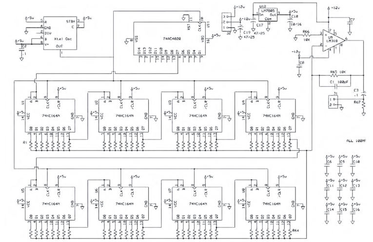
Oscillator Circuit
The way this circuit works is at first all of the outputs are low giving zero volts out. Then at the next clock cycle the first output goes high to 5V. The rest stay at zero. The first resistor causes the output to move up a bit. Then at the next clock cycle outputs 1 and 2 are high giving a greater output. This continues until all the outputs are high and the peak of the sine wave is reached. Output 1 goes low starting the downward journey.
Selecting the right resistor values gives me a good approximation to a sine wave. Note that the voltage reference is the actual power supply voltage. Here I use a common 7805 type regulator. My experience tells me that although many manufacturers make them, they are not all equal. I will not use the cheapest part here. By using a clean 12V source to feed the regulator, the regulation and noise seem to be adequate.
If you use all CMOS logic devices, much of the current draw is used by the regulator chip. Both my oscillators combined drew only 45mA. The classic transversal filter works by multiplying each output by a carefully calculated constant to produce a filter. Because the resistor values are only within 1%, it seems reasonable to use around 100 steps for the filter. My good binary choice was 128, which was easiest to implement.
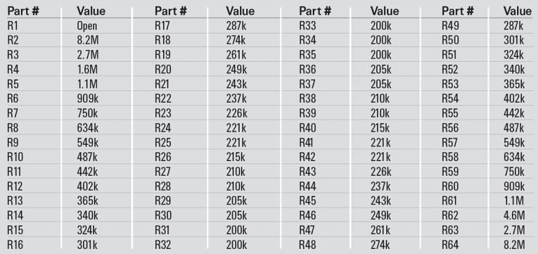
The results of all of these multiples are summed to form the correct value (voltage) by a single op amp. The result should be a sine wave made up of 128 segments. The distortion of this waveform will be mostly determined by the lack of accuracy in my multiplier. In other words, the resistors’ tolerance determines the distortion. Using 1% resistors for the values under 1MΩ and paralleling them reduces the individual contribution to the total error. I would expect this distortion to be less than .25% for the values used here. A simple low-pass filter in the feedback of the op amp should make sure this distortion is lower.
The same filter taps are used for both the positive- and negative-going excursions of the waveform. As a result, the even-order harmonics are very effectively cancelled. The second-order product is almost 95dB down. The highest distortion product is the third harmonic, which is down by 55dB. This is a distortion of .18%. There is also a bit of clock noise that comes through but it is even lower and way out of the bands we are looking at. You could add a filter to lower this, but I wouldn’t bother. Figure 1 is the actual oscillator circuit. You will need two of these.
Components
I used a golden oldie for the op amp — an LM318, which has the slew rate to work for these levels and frequencies. One limit of this op amp is the power supply rejection ratio (PSRR), which is typically 80dB. Each oscillator was fed through a low noise, low distortion 1K resistor to a common 100Ω mixing resistor giving a source impedance of 80Ω. This is close to some guitar pickups and to the 75Ω design impedance of an RCA connector.
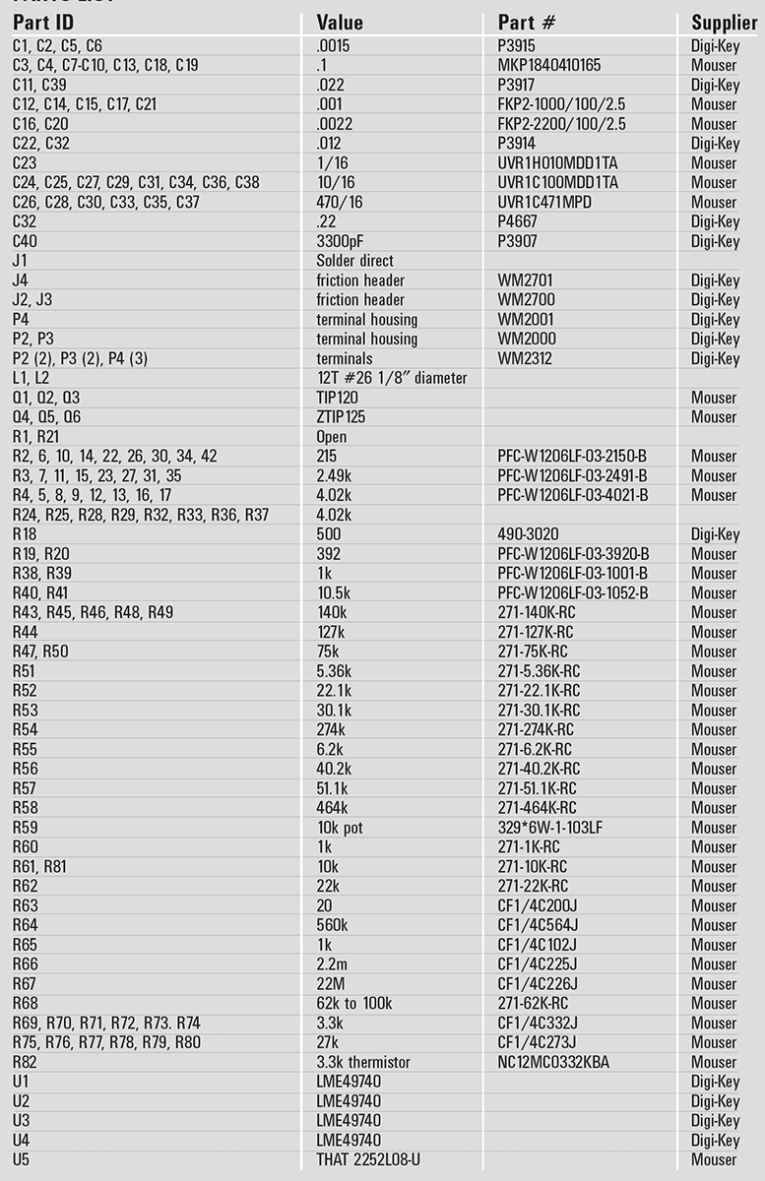
At this point you already have some distortion just from the very small bit of nonlinear or non-ohmic behavior that is in all resistors. This is related to the temperature coefficient of resistance but is also influenced by other factors. The parts list shows the exact critical parts used for my meter.
A source impedance of 80Ω also has an internal thermal noise source equal to the square root of a constant times the absolute temperature times Boltzmann’s constant times the resistance times the bandwidth. The calculation at room temperature is SQRT(1.61 E-20 × R × BW). This is often expressed as nV√Hz ½. For our source this would be 1.14nV for a 1Hz bandwidth.
I chose a low-noise op amp — the National Semiconductor LME49740, which typically has 2.7nV√Hz ½ of noise around 2250Hz. At first I tried a higher noise op amp, which just did not work. The random noise in a circuit adds up according to the square root of the voltages present. You can build a circuit with more than one amplifier on the input signal. All of the outputs will be summed together. The signals add as they are all in phase, with the noise following the square root rule. As a result, there is an improvement in the signal-to-noise ratio equal to the square root of the number of amplifiers used. With four amplifiers the noise drops in half.
The feedback resistors also make noise. So keep these values as low as possible, but not so small the op amp cannot drive them. Another area of concern is removing any RF interference. I did not do this at first, and even some passing cars would cause the meter to clip. I used small film capacitors here along with a small inductor. I just wound 12 turns of 26 gauge high-quality magnet wire around a 1/8″ Allen wrench. This was about the same size as a resistor when finished.
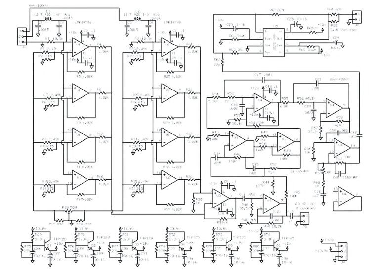
The difference this filter made was quite impressive. The first four op amps of U1 and U2 are just the first stage of an instrumentation amplifier. I used surface-mount tantalum nitride .1% resistors for this stage. U3’s first op amp sums these signals and in effect gives a gain of 50 for the target signal. A balance trim resistor R18 is provided to tweak in the balance. The second op amp of U2 is a 50× gain stage and sources the lightly band-passed signal for the filter stage and for the analyzer output via J3.
The first filter reduces the bandwidth of the signal I will actually measure. This stage does most of the filtering. It uses the last two op amps of U3. The resistor and capacitor values are critical for the center frequency of 2250Hz. No tuning is necessary if the resistors are 1% and the capacitors are 5%. The filter also provides a gain of about 10 to the center frequency. This filter stage is followed by a simpler second bandpass filter consisting of two more op amps in U4. This stage also provides about 100× gain. It is followed by a plain vanilla gain stage with just a bit of high frequency rolloff. This is where you can use any desired scaling. This is the last op amp used in U4 and provides voltage gain of 2 to 11x.
In the last stage a high-pass capacitor feeds a resistor used as a voltage to current converter. This feeds a THAT 2252 true RMS detector chip, which gives an output voltage of 6.2mV per dB. This can be positive if you are above zero reference level, or negative if you are below it. You can use R59 to adjust for an accurate zero reading. R68 and R82 convert the output voltage back into a current to feed the 50μA panel meter. R82 is a thermistor used to provide temperature compensation. The values used give a 25dB meter range.
I used an analog meter on the output. With the distortion component so close to the noise level, the meter swings a bit, and it is much easier to read an analog meter with noise than a digital one. Because I went to a bit of trouble keeping noise out of the circuit design, it is vital to keep the power supply quiet. With the oscillator having a PSRR of only 80dB typical and the analyzer ICs only 60dB at test frequencies, this could be an issue. Batteries are among the quietest source. Lead acid is among the best of the batteries. Noise on the power supplies will show up in the output. I know! I used two completely isolated supplies. For the analyzer board capacitor multipliers, isolate the gain stages.
The only common connection is at the ground point of the mixing resistor. A trickle-charge circuit is active when you switch the meter off. I did not design this unit as a regularly used gizmo. A better charging system would be required if you plan to keep it plugged in.
A 16-gauge steel case housed my instrument. There are internal partitions shielding the oscillators from the detector amplifiers and the power supplies. Even with the shielding there is some leakage!
For the most sensitive uses you may wish to place the instrument and the test item inside a Faraday shield. For input and output connectors I first used a 6-32 threaded brass rod in a plastic insulator. But later for ease of use I changed these to Neutrik RCA connectors.
To tune the meter you can use a short silver jumper and a spectrum analyzer. Insert the jumper and adjust R59 until the panel meter is at half scale. Then adjust R18 for a minimum reading. Using the spectrum analyzer, see how many dB the spike at 2250Hz is above the background noise and adjust R59 until the meter reads twice that. (I did not replace the meter’s scale, so 50μA equals 25dB of distortion above the noise floor.) If you do not have a spectrum analyzer, test all of your RCA cables and set the best one to read 10μA or 5dB — you will not be far off. Figure 2 is the finished analyzer circuit.
Lessons Learned
This instrument is difficult to build and make work reliably. I have provided parts lists. The ground wiring is most important to prevent contamination of the signals. My prototype showed me that some of the components I used were not good enough, so I needed to replace them. I used IC sockets on the first version. The second time I did not use them on the input ICs. The ground wire that goes from the measurement card to the mixing resistor
changed from 18 gauge wire to a piece of ½″ wide copper foil. Finally, this became a piece of silver wire. The input leads are both silver wire the exact same length. One goes to the send jack, the other to the receive one.
Be sure to turn the meter on before you connect a new test cable. The turn-on spikes will change the path measurement if you do not do this! The op amps do heat a bit, so allow the meter five minutes of warm-up to get more consistent readings.
As to the actual use of the instrument, I do not get a perfectly clean reading. The meter jumps a bit even when the connections are working well. Bad connections and cables give nice high readings. Computers, radio transmitters, passing cars, and just about any electrical noise source may cause the meter to jump. I use it on a wood table away from the AC outlets with the lights out and wait for the meter to settle. With some patience you will find you can get repeatable and reliable readings. Looking at the results with a spectrum analyzer shows more insight into what is going on in the cables.
Some have more noise, others more distortion. If you build one of these testers, I hope you will find as I did that the readings do seem to correspond with what you hear. If you are curious as to some of what I learned, one of the first lessons was if you twist a brand new connector around after inserting it, the reading will go down.
That may explain why every time you connect a new piece of gear your system sounds better. A simple experiment you can try is to listen to your system, then unplug and re-plug everything five times. This should make your system sound better!
The second lesson concerns Caig Deoxit, which I have used to fix many noisy or even bad volume controls, touch switches, and even remote controls. I applied a bit to a noisy patch cable under test and nothing happened! I left to do a bit elsewhere and when I returned the noisy cable had become much better. So, Deoxit works, but it takes a bit of time to react!
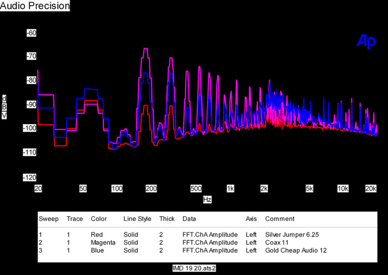
I decided to test some inexpensive RCA-RCA cables I had on hand. Figure 4 shows three different cables. One is a short silver jumper with decent gold RCA plugs. It reads 6.25dB above the noise floor on the meter and has the lowest noise and distortion. The second is a video coax with cheap gold RCA connectors. It has much more noise and distortion and reads 11dB on the meter. The last is a cheap audio cable with cosmetic gold-plated connectors. It reads 12dB on the meter. So there really is a correlation between how you build cables and the test results.
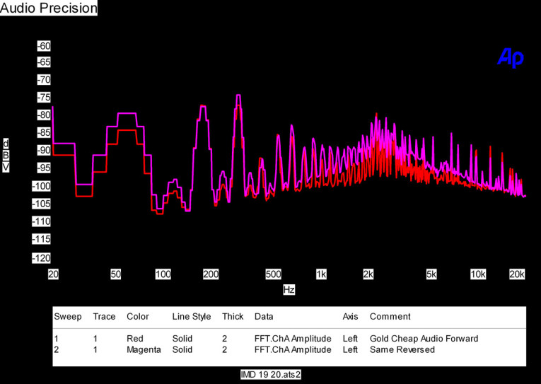
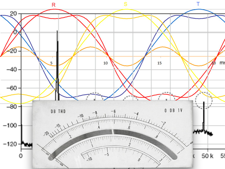
If you look closely at the test results in Fig. 5, you notice the effects of cable directionality. Sometimes, after taking a reading, I turned the cord around and read a different value on the meter. The spectrum analyzer shows why.
Surprisingly, audio cables really do work better one way! To see whether this difference really was there, I used a two-cable switch on my test setup: a Sony CD player through a custom resistive volume control to my custom class A amplifiers into my corner horns. There was a noticeable difference in the apparent high end. Even my secretary noted one sounded louder than another! (Of course, I used the cable that tested for the most change.)
Here are some of the lessons learned:
• Solder connections were at least 50 times better than the best plain mechanical connectors.
• Gold connectors mating to gold connectors work best.
• Shiny (chrome, nickel?) connectors mating to gold are not quite as good — when clean and newly inserted — but become worse within hours.
• Shiny plugged into shiny is not as good as gold on gold.
• Some gold cords made for video and audio were horrible.
• Putting a surge through a cable lowers the distortion for a time, but it comes back. (Maybe the needle drop noise was good for hi-fi!)
As a test of these results, you may choose to replace internal connectors in your gear with straight solder joints, or at least put in a drop of Deoxit. IC sockets in your projects may not be a good idea; at the very least use the gold-plated ones. When doing listening tests, be sure you are not just listening to connector changes. I found I could hear differences of five units on this scale, which is less than the difference between clean and dirty connectors.
The distortion that is being measured is at low signal levels. Pro gear works at level of 0dBm, which is higher than consumer gear, meaning the percentage of distortion will be lower. The load impedance is also lower. You may prefer to try higher levels out with your gear and lower power amplifier gain.
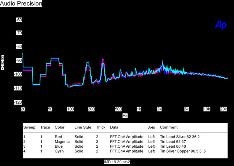
The final results on solder are shown in Fig. 6. I just don’t see any significant differences. 110 solder joints and it still is better than 6" of silver wire! It may be too late for Brian, but I suspect that if he had cleaned his overheated connectors and removed the oxide that had built up on them, they may have sounded fine. aX
This article was originally published in audioXpress, November 2009