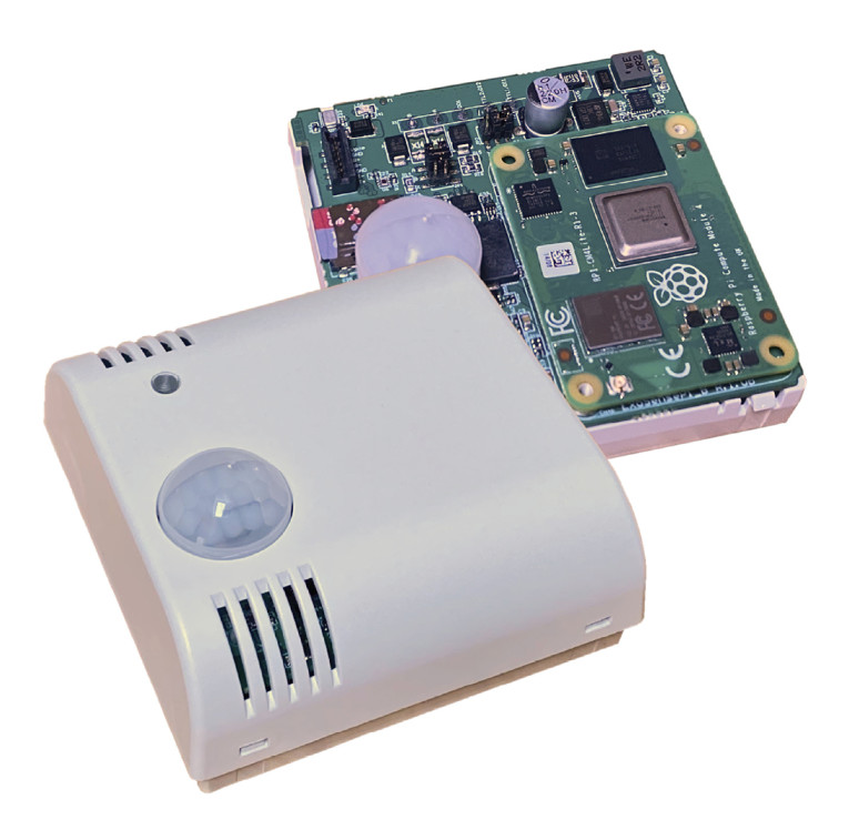
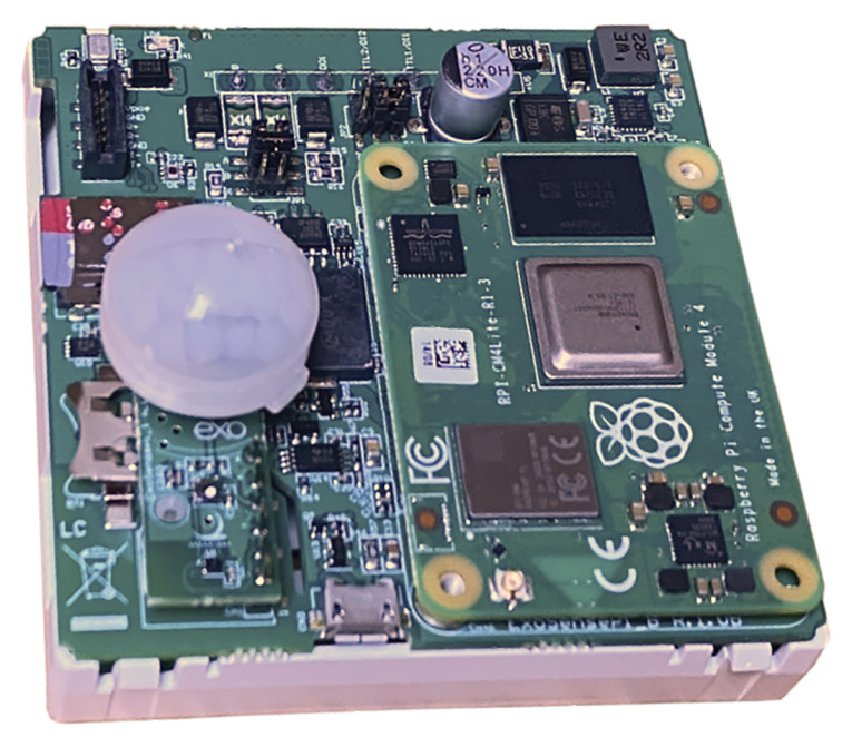
In addition to audio recording, the microphone can also evaluate ambient noise levels, simulating the behavior of a sound meter. Unfortunately, software and documentation about noise level evaluation are scarce online, so we developed and integrated its software to be used with the Exo Sense Pi (Photo 2).
This article will share the knowledge gained by Sfera Labs, illustrating the main concepts involved, hoping to provide guidance and help to those who intend to develop or integrate software applications regarding sound level evaluation with Raspberry Pi.
Sound Pressure Level (SPL)
Humans perceive the sound using the eardrum, a membrane that vibrates after a pressure change due to oscillations of the particles in the air that surround us, providing the sensation of hearing.
When a solid and elastic object (e.g., a tuning fork) is stressed mechanically due to collision, it starts to vibrate. The collision acquires potential energy, which is transferred to the surrounding air particles as kinetic energy, making them vibrate around their static equilibrium position.
The measure of the over-pressure produced by the acoustic perturbation, in each time instant t, can be called p(t). Because of the enormous range of sound amplitude, the pressure is used in logarithmic form, multiplied by 10, and compared to the reference acoustic pressure p0=20μPa. The value of 20μPa is the absolute audible threshold for a typical human listener for a pure tone sound with a frequency of 1,000Hz (often considered as the threshold of human hearing, roughly the sound of a mosquito flying 3m away).
Since in sound level evaluation what is essential is the energetic significance of the sound field, the formula to compute the instantaneous sound pressure level (SPL) in decibels (dB) considers the square of the acoustic pressure instead of just the acoustic pressure:
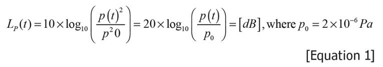
Intuitively, some may wrongly think that if decibel describes the SPL, then 0dB means a state of no sound present. Decibels measure a ratio: 0dB does not mean sound absence; it means a sound level equal to that of the reference level p0:

p0 is a small pressure, but not zero. It is also possible to have negative valued sound levels (e.g., -20dB would mean a sound with pressure 10 times smaller than the reference pressure p0).
Equivalent Continuous Sound Level (LEQ)
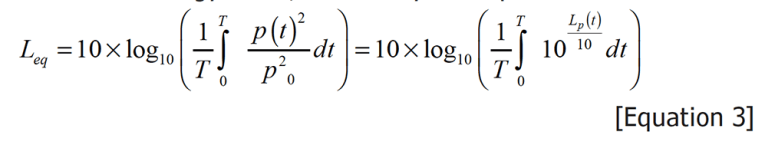
In electric systems and sound level evaluation processes, the RMS value is preferred to the actual value to indicate the quantity of noise/energy over a certain period. For example, in electrical engineering, the RMS value of an alternating current passing through a resistance is the value of a direct current that causes the same increase in the temperature of the resistance in the same period. For sound evaluation, the RMS (also called Equivalent Continuous Sound Level or LEQ) is the SPL value of a constant sound over the same period, which produces the same amount of energy/noise, defined by the equation:

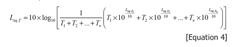
The use of the LEQ is also very convenient for math operations because it is possible to add the LEQs of different periods and get a resultant LEQ value for the total of all periods, according to this equation:
Time Weightings as Classifiers
After finding the way to measure and quantify the SPL, scientists of the past asked themselves if it is also possible to recognize particular types of sounds. They made tests whose empiric results can provide a general indication about which time constants to use to recognize different classes of sounds:
- FAST time constant = 125ms. Used to replicate the natural response of the human ear.
- SLOW time constant = 1000ms. For environmental noise studies, especially for studies that span many hours or even days, because it is good at “ignoring” short, fast sounds (e.g., a door slamming or balloon popping).
- IMPULSE time constant = 35ms. Used in situations where sharp, impulsive noises are measured (e.g., fireworks or gunshots).
Frequency Weightings
Human eardrums are different from those in other species, and they have their distinct properties and behaviors. Humans can hear sounds up to the frequency of 20kHz, while dogs can hear up to the frequency of 45kHz.
We made speakers and microphones by imitation based on the same principle of the vibrating membrane as the eardrum. Unfortunately, they cannot perfectly replicate the different responses of the human ear to different sound frequencies because the human ear is less sensitive to very low or very high sound frequencies. The solution is the use of frequency weighting tables.
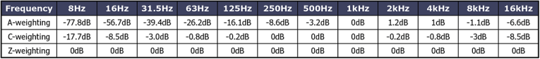
Sound frequency adjustment tables are a collection of sound level adjustments values for frequency bandwidth intervals, usually of 1 octave or fractions of octaves, applied during the sound evaluation. Three types of the most used frequency weightings are:
- A-weighting (unit of measure dBA): Used to replicate the behavior of the human ear
- C-weighting (unit of measure dBC): The C-weighted sound level does not discriminate against low frequencies and measures almost uniformly over the frequency range between 31.5Hz and 8kHz. This scale is helpful for monitoring sources such as engines, explosions, and machinery.
- Z-weighting (unit of measure dBZ): No frequency weighting is applied.
Table 1 shows an example of a one-octave frequency weighting table. For example, in A-weighting, the LEQ representing all the sound components with frequencies between 0Hz and 8Hz must be adjusted, adding -77.8dB. In comparison, -56.7dB is added to all the components with frequencies between 8Hz and 16Hz.
Microphone
The basic hardware to implement a sound evaluation system is a microphone connected to a central computation unit. In the specific case of Exo Sense Pi, the computation unit is the Raspberry Pi, and the microphone is the ICS-43432 digital microphone (Figure 1).
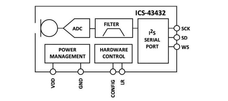
The ICS-43432 microphone offers multiple advantages including: Suitable sampling frequencies up to 52.8kHz (humans can hear up to 20kHz, so according to Nyquist sampling theorem, a minimum sampling frequency of 40 kHz is required to emulate human perception of noise); digital discrete output; easy audio samples configuration and retrieval using a I2S communication interface with Power Code Modulation (PCM) data representation and Linux ALSA audio drivers; low sensitivity error (±1dB); no need for calibration; small and compact dimensions; and easy integration with other devices.
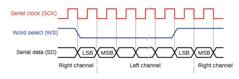
I2S is an electrical interface used for audio data transmission. It is composed of one or more lines for data transmission; a line used to mark individual bits called “bit clock”; and a line used to delineate frames tolled “word clock” (Figure 2).
Instantaneous SPL from Microphone
A crucial task is the reading of the actual sound pressure from the microphone. In order to perform this operation correctly, we used the following information from the datasheet:
Data format: ICS-43432 can be set to use 24 signed little endian digital format. In this case, the first bit is the sign, then the maximum digital value in output is 2^23 = 0x7FFFFF = 8388607
Sensitivity: It expresses a microphone’s efficiency as a transducer (how well it converts acoustical energy to electrical energy). A microphone’s sensitivity rating is due to its output voltage related to its measuring SPL. The standard reference input signal for microphone sensitivity measurements is a 1kHz sine wave at 94dB SPL (equivalent to 1 Pascal). ICS-43432 microphone has a sensitivity value of -26dB, compared to a 1kHz sine wave at 94dB or 1Pa SPL.
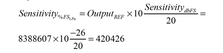
For digital microphones, sensitivity is a percentage of the full-scale output generated by a 94dB SPL. For a digital microphone, the conversion equation is:
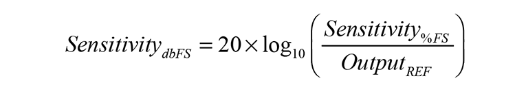
where, OutputREF is the full-scale digital output level. As written above, in the specific case of the ICS-43432 microphone, the sensitivity is -26dB, and the full-scale digital output level is 8388607, so our equation becomes:

from which we can compute the exact digital value to represent 1Pa SPL:
Now it is possible to interpret any reading from the microphone and compute the instantaneous SPL in Pascal (Pa), using the following equation:

Software Architecture
The noise level evaluation process is complex because it involves a large set of software. On Exo Sense Pi and Raspberry Pi, the Linux operating system offers tools (e.g., the ALSA libraries) for sound card management or libraries to perform Fast Fourier Transforms (FFTs).
There are different ways to implement the same sound evaluation procedure using different software. Figure 3 illustrates the basic software structure implemented inside Exo Sense Pi, using ALSA audio drivers.

The main idea behind this architecture is the creation of a core Linux software application, called soundEval, which main functions include: set up microphone configuration (sampling rate, audio data format, channels); retrieve instantaneous SPL from the microphone; and perform sound evaluation accordingly to evaluation parameters, such as time weighting constant, frequency weighting type return evaluation results.
The soundEval application is designed to be run on any Linux OS (Figure 4). The Exo Sense Pi kernel module works merely as a device-specific interface between the end-user and the soundEval application, to facilitate the use of evaluation procedures by the end user, like the automatic configuration of the microphone in the Exo Sense Pi.
Exo Sense Pi and Sound Evaluation
The simplified flow chart with sound level evaluation steps implemented in Exo Sense Pi is shown in Figure 5.
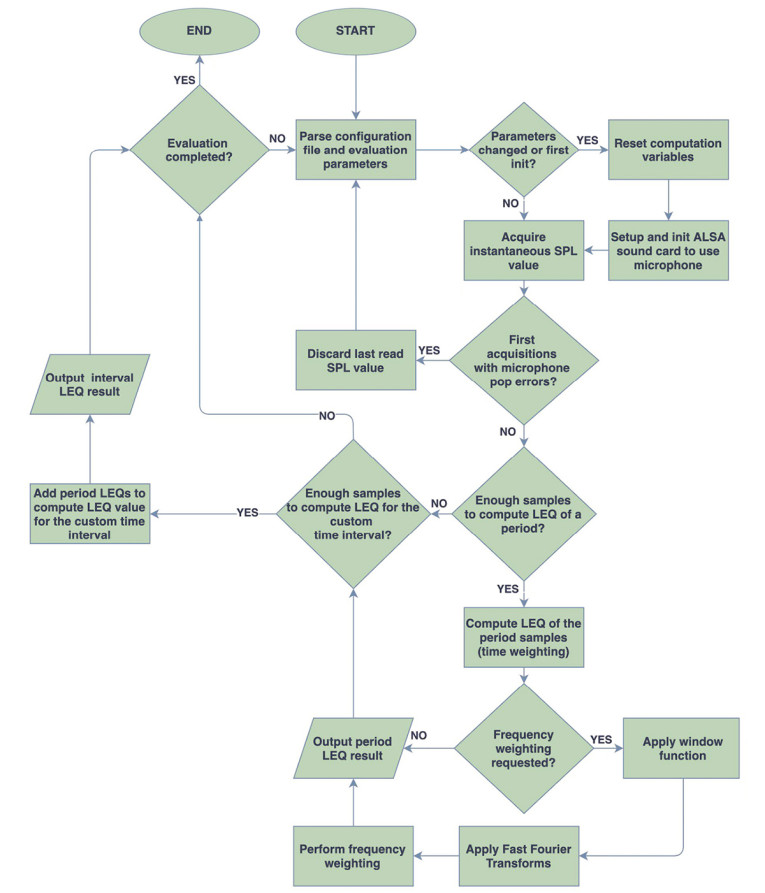
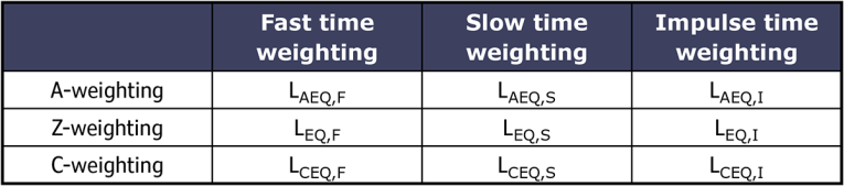
Table 2 shows the combination of different time constants and frequency weightings, which provides results of different classes of sound meters.
Depending on the requirements of an application, it is possible to use the sound level evaluation as a classifier and a LEQ calculator.
One example of sound evaluation as a classifier is the explosion detection in a chemical materials storage facility. An LEQ evaluation with IMPULSE time constant and frequency C- weighting can detect explosions if the LEQ of a period of 35ms exceeds a threshold dBC value.
One example of sound evaluation as an LEQ calculator is evaluating the equivalent sound level generated by a music concert using an A-weighting frequency adjustment. After computing the LEQ for the entire concert duration, it is possible to compare this result with threshold values and check if the concert volume level was compliant with local regulations.
Since frequency weighting is involved in sound evaluation processes after applying the FFTs, it is possible to return the LEQs of a period, split up by frequency bandwidths, typically of 1 octave or a fraction of octave. With this capability, it is possible to perform operations, such as the creation of a graphic audio spectrum real-time display; a search for bandwidths in which the noise is mainly concentrated, for noise-canceling procedures; and a more detailed sound classification, which also considers the LEQs of each frequency bandwidth.
Conclusions
The soundEval application is an easy to use utility that implements the recognized sound level metering standards, based on an audio feed from a digital microphone. Besides its use in Exo Sense Pi, it could also be used with other hardware platforms, and adapted to process pre-recorded audio or network streams instead of a directly connected digital microphone aX
Resources
“Octave band,” Wikipedia, Wikimedia Foundation, May 11, 2020,
https:// en.wikipedia.org/wiki/Octave_band
“Pulse-code modulation,” Wikipedia, Wikimedia Foundation, July 5, 2021,
https://en.wikipedia.org/wiki/Pulse-code_modulation
“Spectral leakage,” Wikipedia, Wikimedia Foundation, November 17, 2020,
https:// en.wikipedia.org/wiki/Spectral_leakage
“Window function,” Wikipedia, Wikimedia Foundation, August 20, 2021,
https:// en.wikipedia.org/wiki/Window_function
This article was originally published in audioXpress, March 2022.
 About the Author
Ben Chen holds a bachelor and a master degree in “IT engineering” at “Politecnico di Milano.” He has extensive working experience as a software engineer, mainly in developing automation applications for plastic production/packaging/wire drawing machinery. Ben is also a music lover and a maker.