
In Part 1 of this article we discussed the key features of Virtual Voice Coil (VVC), software used for designing voice coils and easily predicting audio transducer parameters. We left off with the SPL chart, bottom right of Figure 6, with the cursor aligned with the darkest bar. The darkest bar represents the maximum value among all wires. So, this is the maximum SPL, but is this also the maximum efficiency of the system?
As we can see from the bottom left graph of Figure 6, the cursor in the Wire Loss chart is not aligned with the darkest bar. The darkest bar in the Wire Loss chart indicates the highest efficiency among all wires that is the golden ratio linked to the selected voice coil electrical and mechanical parameters and independent of the magnetic flux. When both the two cursors are not aligned with related dark bars, it means the potential efficiency of the system could be improved. Operating with some minor adjustments and using the two cursors alignment as target, doubling the number of layers and selecting a Ø0.4 mm wire, now the two cursors are both aligned over the dark bars: this is the maximum achievable system efficiency!

As visible in Figure 7, Bl passes from 16 to 24 Tesla (T) per meter, the SPL passes from 73.52dB to 74.32dB, so we have added +0.8dB and the voice coil inner diameter is bigger than 46.5mm, thus the voice coil is physically feasible, while gaining the maximum efficiency of the system.

Using a Magnetic Gap
In the last example, a magnetic circuit without a magnetic gap has been used to have the maximum degree of freedom for the voice coil’s outer diameter (OD). Using the presented method (both wire size cursors aligned over the darkest bars as the target), it is possible to obtain the maximum efficiency for a loudspeaker with a magnetic gap, in this case, if practicable, it could be necessary to also work on the motor design, importing magnetic flux density variations due to OD restrictions.
Regarding this topic, an important value to consider for the voice coil is the mean diameter, because if we set the mean diameter, it represents a fixed value for the FEA magnetic cut line. No matter if we change wire’s dimension or layers number. In the first loudspeaker simulation from Figure 6, the inner voice coil diameter is 50mm. Keeping the inner diameter of Figure 8, if we change wire section to 0.4mm and number of layers to 12, we obtain a new mean diameter = 55.268mm, as shown in Figure 9.


But 55.268mm, is not the correct diameter of the imported FEA magnetic cut line of Figure 6 and Figure 8, indeed, the density flux cut line at Ø55.268mm is completely different. Figure 10 shows a B(x) comparison. The average flux, along a voice coil with 10.365mm height, pass from 0.518T to 0.417T, giving a reduced Bl(x) and dBSPL with different Thiele-Small (T-S) parameters. As a new feature, in VVC 2.1, it is possible to switch between inner and mean diameter. Indeed, in Figure 7 is fixed the same mean diameter (55.202mm) of Figure 6. Fixing the mean diameter ensure the voice coil position remains the same, regardless, for example, of wire size or layers number changes and it is possible to compare voice coils using the same magnetic flux density cut line.

Asymmetry Graphs
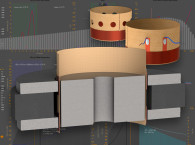
Now we can see how to practically use Bl(x) asymmetry graphs, designing, for example, a typical loudspeaker motor in Figure 11, with a 25mm voice coil diameter and Y-30 Ferrite (84mm×32.8mm×15mm). A flat nucleus diameter of 24.4mm and an upper plate diameter of 26.73mm plotting flux density, with FEA software, along the line crossing magnetic gap, and representing the available voice coil displacement. Then importing the flux density profile into VVC (considering that both period and comma decimal separators are accepted). At the moment, we can neglect loudspeaker parameters, they are not important for the symmetry analysis we are going to do. Adjusting the offset, it is possible to gain a better symmetry compromise with a new rest position with offset = -0.55mm, as shown in Figure 12.


In Figure 13 we can observe a good symmetry for excursions >5mm. But the symmetry is not good for displacements inside the Blmin = 82%<5mm. As we already know, extending the nucleus as in Figure 14, it might help to symmetrize flux.


Importing flux and shifting offset = 0.03mm, total asymmetries = 0.11% are now, in Figure 15, about one order of magnitude lower than the flat nucleus.

Observing Figure 16, the two curves in Bl(x) graph seem overlapped, but as we can see from Bl(±x) Offset Asymmetry graph, we still have some peaks of about 0.2% and total asymmetries = 0.11%. Moreover, the Bl (±x) Rest Position Asymmetry graph shows some oscillations with a rest peak of -0.27mm.

Now if we modify the nucleus extension with a sloped uppercut as shown in Figure 17, importing flux and shifting offset = -0.13mm, we obtain the best symmetry for this motor design, as visible in Figure 18. Reducing Bl(x) asymmetries for the full displacement of the voice coil with a flat Bl (±x) Offset Asymmetry curve, see Figure 19, and the minimum total asymmetry recorded 0.09% among the various designs. The Bl(±x) Rest Position Asymmetry is also improved using the sloped uppercut, less oscillations and a reduced amplitude, it is now -0.15mm. These are some simple examples just show how to use VVC asymmetry graphs for optimizing a loudspeaker motor design.


Additional VVC 2.1 Features
In the new VVC version 2.1, it is possible to add more than one spider (maximum three spiders), then surround and spider rates measure their contribution on total system. When the Cms window is expanded for the first time in VVC, the default value of the surround rate is 20% of the total Cms or Kms and the spider rate is 80%. It is a suggested starting point, also suggested by Vance Dickason in the Loudspeaker Design Cookbook 8th Edition.
Another feature of VVC 2.1 is the Transducer Cable Loss, which refers to the cable from amplifier to loudspeaker terminals. Cable loss is suitable for dimensioning cables in a project, controlling, for example, SPL reduction or how the Loss Factors will change. VVC automatically recalculates related loudspeaker parameters. For the cable core material, four options are available, and its electrical conductivity is referred to the air temperature (Temp) at which the transducer is measured. We can set the cable diameter, or we can set the American Wire Gauge, or the core section. To preserve the right quantity of total damping, it is an important value to consider, to control back EMF of the transducer’s moving masses, especially in subwoofer applications.
Finally, VVC 2.1 offers three options for Voice Coil Wiring, selecting a single voice coil as standard configuration, or it is possible to combine two voice coils in parallel or in series. A new video tutorial about VVC is available on the www.speakerlab.it website, which provides more examples of the material presented in this article. VC
Read Part 1 of this article here.
This article was originally published in Voice Coil, March 2025