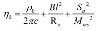
SpeakerLAB Virtual Voice Coil (VVC) is the ideal software for designing voice coils and predicting audio transducer parameters with maximum accuracy in an easy way. One of the keys that allow the accuracy of VVC prediction is given by a complete temperature management involved in loudspeaker calculus. For a precise calculus of loudspeaker parameters and the sound pressure prediction in the far field, based on a linear model and assuming a radiation in a half space (2π-sr free field), it is necessary to recognize temperature interactions among the terms of the reference efficiency formula of electro-acoustical conversion:
In reality, there are three kinds of temperatures for defining loudspeaker efficiency and thus the reference sensitivity in the loudspeaker pass band.
The First Temperature
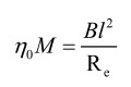
The first temperature is linked to voice coil winding and in VVC it is called wire temperature (wTemp). It represents the environment temperature at which the voice coil is assembled. In other words, it is the temperature of the supplier factory during voice coil winding phase. By the wire temperature VVC defines primary electrical resistance included in Re, moreover the materials thermal expansion, the wire length l with a partial stretch and wire section variation. Thus, wTemp has an effect on Mms and both Bl and Re, involving the motor efficiency factor term in the efficiency formula:
The Second Temperature
The second temperature is linked to the environment working temperature at which the transducer is measured, it is called air temperature (Temp). It is important if we are measuring DUT at a different temperature, or for example, we are going to install the loudspeaker in a different temperature due to environment conditions and we want to know the final sound pressure level or parameters variation. Temp involves the first term of the efficiency formula (because of the air density ρ0 and the speed of sound c) and the third term of the efficiency formula, because Mms includes the mechanical mass Mmd and air load mass (which varies with air density ρ0 and consequently with the temperature Temp).
The Third Temperature
The third temperature, available only in VVC 2.1, is ∆T (expressed in Kelvin) and it is related to voice coil temperature increase, due to Joule heating. Moving ∆T slider, VVC recalculates in real time all involved electrical parameters, as the DC resistance and related electric power and current variations, or some acoustical parameters, as the transducer sensitivity decibel sound pressure level (dB SPL) reduction (due to power compression) or Loss Factors variation.
Moreover, VVC also calculates mechanical parameters variations due to Joule heating, as the voice coil winding height (H), the minimum inner diameter or maximum outer diameter, due to materials thermal expansion. This tool is very helpful for evaluating and optimizing clearances inside the magnetic air gap. VVC computes parameter estimation assessing these three kind of temperatures, obtaining very accurate results.
Expressions for Temperature Dependent Parameters
To develop expressions for all temperature dependent parameters, the following assumptions are made: resistivity and dimensions vary as a function of temperature, depending on geometry, material thermal expansion, coefficient of thermal expansion, material temperature coefficient of resistance, material thermal conductivity, material electrical resistivity. Particularly resistivity and thermal expansion are linear functions of materials, respectively:
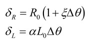
where ξ is the temperature coefficient of resistance, R0 is the original resistivity, α is the coeffcient of thermal linear expansion, L0, is the original length. For both expressions Δθ is the temperature variation, including the three temperatures (wTemp, Temp, and ΔΤ), restricted in a range such that ensuring linear functions for wTemp and Temp and using a nonlinear second order function for ΔΤ.
In Joule heating of voice coil wire, using for example multi-layers voice coils, the external layers lose heat to ambient air and subsequently result in a lower temperature if compared to wire wound in an internal layer. This is not achievable with the available VVC input data and for convenience the software doesn’t comprise free or forced convection in air, but heat dissipation by internal conduction only.
So, B and Sd are the unique terms in efficiency formula VVC doesn’t consider as temperature dependent variables. Because Sd is considered as a pure dimensional input. On the contrary, the magnetic flux density B is affected by temperature in reality (with reversible temperatures coefficients and irreversible loss of magnetic assembly), but B variation depends on used magnetic materials and geometry topology information, which are external to VVC data, hence B(x) values are assumed as temperature invariant.
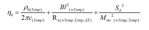
Environment Humidity variable (Hum) is present among VVC inputs, it has less influence in the efficiency formula, thus we can rewrite the temperature dependent η0 as it is treated by VVC:
Now we can see how VVC processes elements simulated and imported from external FEA software. This method is very important for processing data in a reliable way.
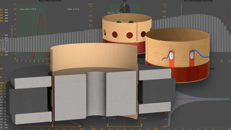
For motor designs with an axis of symmetry it is always a good practice to operate with partial models, dividing them along the symmetry axis and using only a section of the entire model; but for the evaluation of an algorithm behavior related to symmetries a FEA of the whole symmetrical model is necessarily done and imported in VVC, the flux density B(x) is visible in Figure 1. In symmetrical designs, small differences between the two opposite mirror sides of the B(x) and Bl(x) profiles could yield to plots values of asymmetries >0 %.
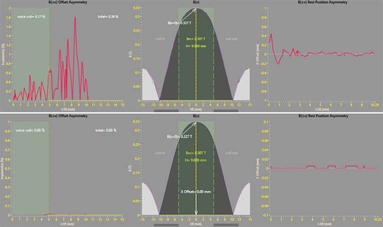
These differences are due to finite element mesh, particularly FEA mesh nodes and their positions in space, and to the geometry of the mesh elements, their dimensions, and distribution. Figure 1 also shows two different mesh element dimensions (with the maximum and the mean value along the B cut line).
When a flux density is imported, VVC operates a resample of B(x) for setting cursor in an independent mode compared to imported x points step, then an automatic weighting filter is applied. Smoothing a curve could be dangerous, sometimes a great deformation of the curve occurs when a smoothing filter is used.
The applied Auto Tune Filter (ATF) depends on inflection points biased to the curve gradient of the FEA imported data. This filter is suitable for reducing errors due to different FEA mesh methods.
A first stage of the filter computes the absolute value of the arctangent of y/x, for angles in any of the four quadrants of the x-y plane, to obtain the curve gradient |m|, measuring the steepness of the curve and inflection points positioned along the curve steepness.
The ATF of the imported magnetic flux density B(x), simulated with external FEA software, is set according to a fitting model which works as a smooth of the data set (X [mm], Y [T]) according to a minimization of the following function:
Auto Tune Filter (ATF)
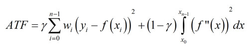
- wi is the ith element of Weight. Weight depends on gradient amplitude.
- yi is the ith element of Y.
- xi is the ith element of X.
- f”(x) is the second-order derivative of the cubic spline function, f(x).
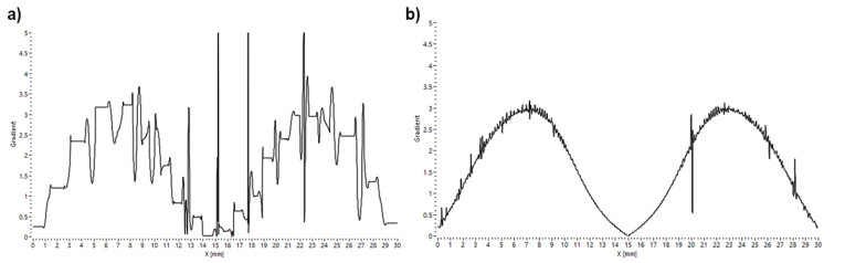
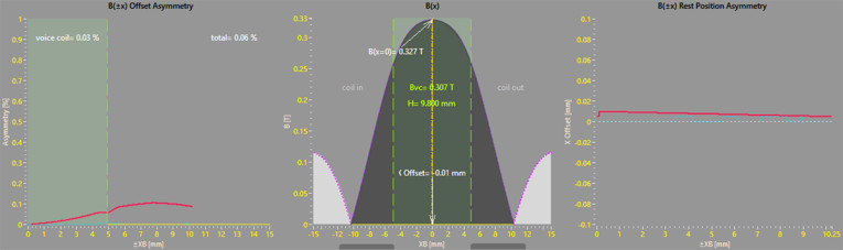
The gradient of the ATF filter is shown in Figure 2, and the results of its application are visible in the bottom image of Figure 1. Using the coarse mesh (2mm max element), applying the ATF filter, and moving the voice coil offset = 0.01mm coil-in, the current (red line) symmetry compared to offset = 0 (dashed blue line) is visible in Figure 3.

In the worst case, using a very coarse mesh, values of asymmetry peaks <0.2% could represent symmetrical ±x points. While using the finest mesh (0.1mm max element) and moving offset = 0.01mm coil-in, its symmetry is now shown in Figure 4 in which is possible to appreciate very small differences.
Anyway, you can test your own CAD-FEA-VVC chain, designing, simulating, and importing a symmetric motor flux density, for examining the symmetry goodness.
Maximizing Loudspeaker Efficiency
After the introduction of some of the key features about VVC data processing, we are going to see a novel technique for maximizing efficiency of a loudspeaker, using VVC Wire Loss and the SPL charts. The Wire Loss chart was presented in 2014 in the first version of VVC, then all bugs of the old version were solved in VVC 2. For instance, a simple symmetrical magnetic circuit, with a 50mm inner diameter voice coil is considered.
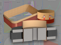
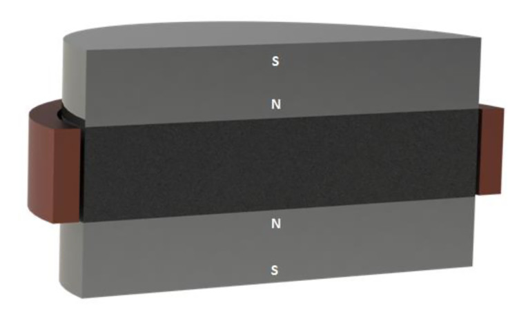
As visible in Figure 5, it is an open-gap magnetic system, with two magnets in mirror arrangement having negative fluxes along the B(x) bounds. The negative values are sampled in absolute value and shown in light grey color in the positive Y. This is convenient for permitting evaluations of applied negative forces (it can be used for electromagnetic breaks) compared to the positive force, along the same voice coil displacement. The voice coil is without a former, only winding, and for the simulation the B(x) flux density cut line is selected to accept voice coils with different diameters.
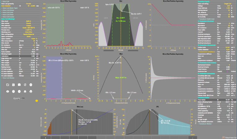
The design can accept 46.5mm as the minimum voice coil inner diameter. In VVC, after importing a B(x) for an air gap length of ±15mm and arranging voice coil data, disabling the former, we can move the wire size cursor over the darkest bar in SPL chart, obtaining the highest SPL of 73.52dB using a Ø0.33mm wire. As we can see from the SPL chart, shown in bottom right of Figure 6, the cursor is aligned with the darkest bar. VC
SpeakerLAB Website
This article was originally published in Voice Coil, February 2025