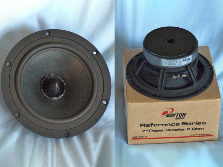
The Dayton RS180-8’s motor design is rather sophisticated and incorporates a copper shorting ring (Faraday shield), a T-shaped pole piece, and an aluminum phase plug. The ferrite magnet motor is finite element analysis (FEA) designed using a 1.5” (38 mm) diameter voice coil wound with round copper wire on an aluminum former. The motor parts, the T-yoke, the front plate, and the bullet phase plug (which also partially acts as an inductive shorting device) have a black heat-emissive coating for improved cooling. (No other vents including pole, peripheral, back plate or vents below the spider mounting shelf are used.) Last, the voice coil is terminated to a pair of gold-plated terminals. Cosmetically speaking, this is very good looking driver.
I used the LinearX LMS analyzer and VIBox to create voltage and admittance (current) curves with the RS180P-8 clamped to a rigid test fixture in free-air at 0.3, 1, 3, 6, 10, and 15 V. As with almost all 6.5” to 7” drivers, the 10-V curves are usually too nonlinear for LEAP to get a reasonable curve fit. However due to the RS180P-8’s linearity and high XMAX, I was able to use all the curves including the 15-V curves. For Test Bench, I no longer use a single added mass measurement. Instead, I used actual manufacturers’ measured Mmd data (11.6 g).
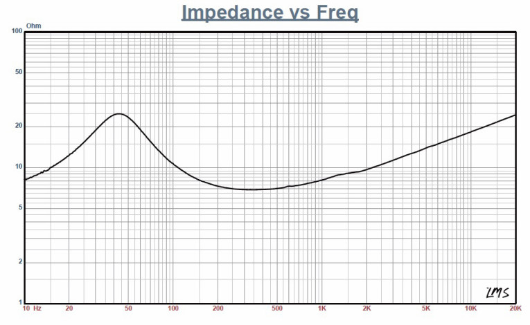
Next, I post processed the remaining eight 550-point stepped sine wave sweeps for each RS180P-8 sample and divided the voltage curves by the current curves (admittance) to derive impedance curves. I used the LMS calculation method to add phase and imported the data, along with the accompanying voltage curves to the LEAP 5 Enclosure Shop software. Since the majority of OEM manufacturers use either the standard model or the LEAP 4 TSL model to generate most Thiele-Small (T-S) data, I used the 1-V free-air curves to create a LEAP 4 TSL parameter set. Figure 1 shows the 1-V free-air impedance curve.
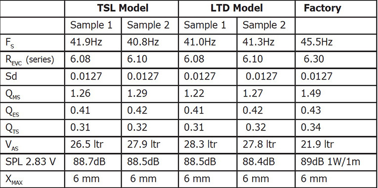
Next, I selected the complete data set, the multiple voltage impedance curves for the LTD model, and the 1-V impedance curve for the TSL model in the transducer derivation menu in LEAP 5 and created the parameters for the computer box simulations. Table 1 compares the LEAP 5 LTD, the TSL data, and the factory parameters.
The RS180P-8’s LEAP parameter calculation results were similar to the factory data. As usual, I followed my normal protocol and used the LEAP LTD parameters for Sample 1 to set up the computer enclosure simulations. I programmed two computer vented box simulations into LEAP 5, one QB3 with a 0.33-ft3 volume tuned to 50 Hz and an extended bass shelf (EBS) vented enclosure with a 0.6-ft3 volume tuned to 41 Hz. Both the enclosures were simulated with 15% fiberglass damping material.
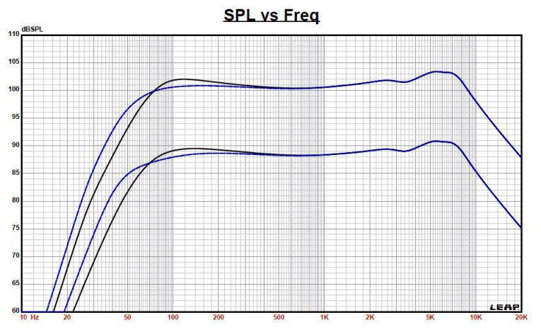
Figure 2 shows the RS180P-8’s results for the two vented boxes at 2.83 V and at a voltage level sufficiently high enough to increase cone excursion to 6.9 mm (XMAX + 15%). This produced a F3 frequency of 68 Hz (F6 = 55 Hz) for the QB3 enclosure and –3 dB = 54 Hz (F6 = 42 Hz) for the EBS-vented simulation. Increasing the voltage input to the simulations until the maximum linear cone excursion was reached resulted in 102 dB at 13 V for the QB3 enclosure simulation and 101 dB for the same 13-V input level with the larger vented box.
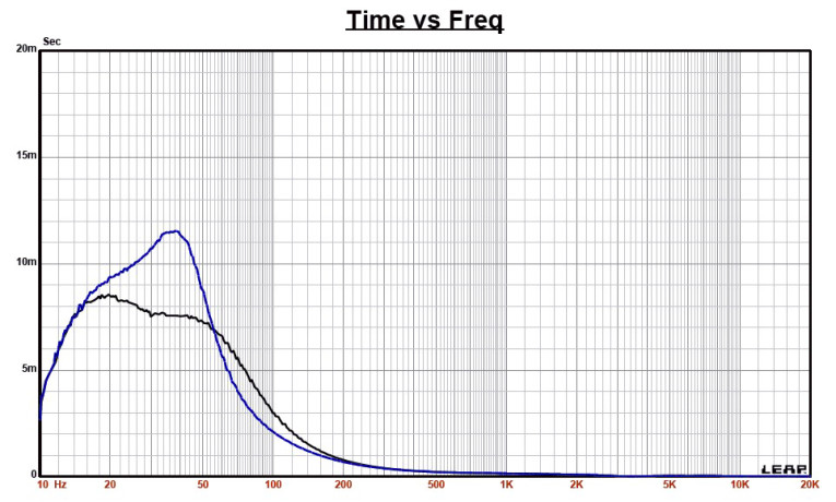
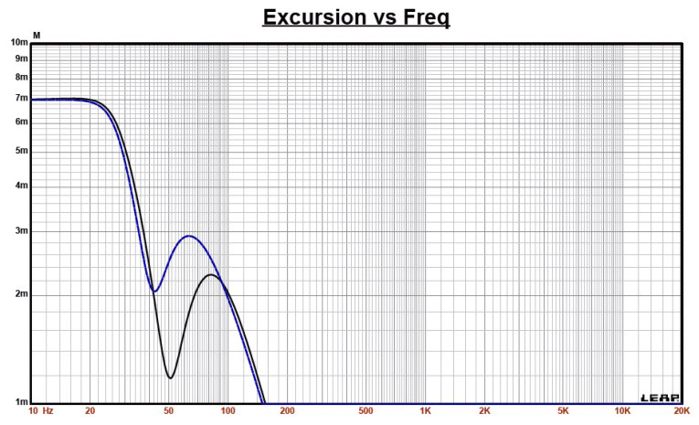
Figure 3 and Figure 4 show the 2.83-V group delay curves and the 13-V excursion curves. Note that because both drivers reach maximum excursion at about 22 Hz, a steep 24-dB/octave high-pass filter located from 25 to 35 Hz would increase the power handling of both box examples by a substantial margin.
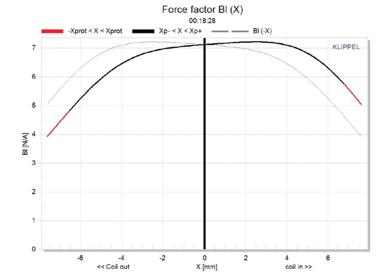
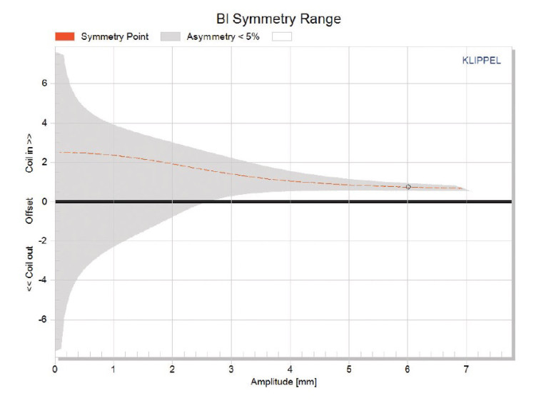
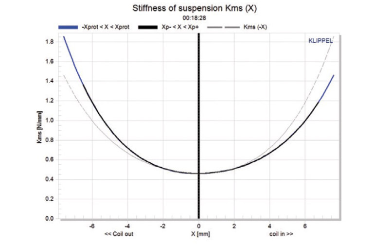
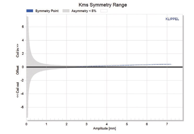
Pat Turnmire (Redrock Acoustics) performed the Klippel analysis. (Our analyzer is provided courtesy of Klippel.) The RS180P-8’s analysis produced the Bl(X), KMS(X), and Bl and KMS symmetry range plots shown in Figures 5–8. This data is extremely valuable for transducer engineering. The RS180P-8’s Bl(X) curve is fairly symmetrical and somewhat tilted, but it is actually a moderately broad Bl curve compared to most 6.5-7” woofers (see Figure 5).The Bl symmetry plot shows a rather small 0.74-mm coil-in offset at physical XMAX position, which is probably within manufacturing tolerance (see Figure 6).
Offset at the rest position did not resolve very well, which is what the large grey area represents. Figure 7 and Figure 8 show the RS180P-8’s KMS(X) and KMS symmetry range curves. The KMS(X) curve is also symmetrical in both directions, with mostly zero offset out to 3 mm and only rising to a small coil-in rearward offset of about 0.35 mm at the physical XMAX position.
The RS180P-8’s displacement limiting numbers (calculated by the Klippel analyzer) were Bl(X) at 82% (Bl = 5.2 mm) and for the crossover at 75% CMS the minimum was 3.2 mm, which means compliance is the most limiting factor for a 10% prescribed distortion level. If we use a less conservative 20% distortion criteria of Bl falling to 70% of its maximum value and compliance falling to 50% of its maximum value, the numbers would be Bl(X) = 6.3 mm and the crossover = 5.
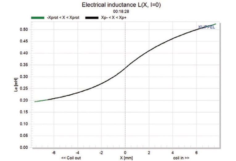
Both numbers are closer to the driver’s physical XMAX. Figure 9 shows the RS180P-8’s inductance curves Le(X). Inductance will typically increase in the rear direction from the zero rest position as the voice coil covers more pole area. However, this inductance does not occur because of the multiple inductive shorting devices (i.e., the copper shorting ring and the aluminum phase plug). The result is a minor inductance swing with inductive variation of only 0.29 mH from the in and out XMAX positions, which is good performance.
Next, I mounted the RS180P-8 in an enclosure, which had a 8” × 15” baffle filled with damping material (foam). Then, I used the LinearX LMS analyzer set to a 100-point gated sine wave sweep and measured the device under test (DUT) on- and off-axis from 300-Hz-to-40-kHz frequency response at 2.83 V/1 m.
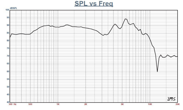
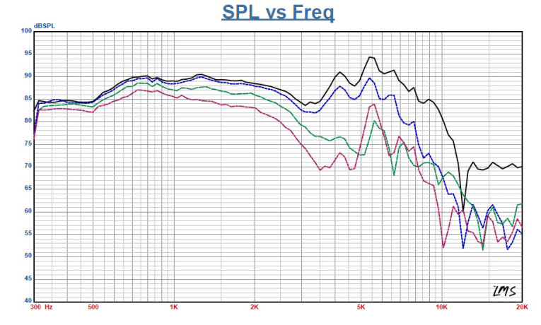
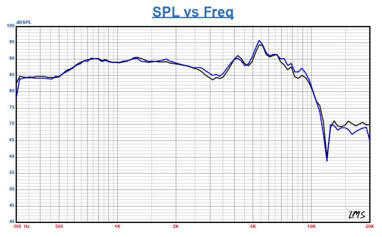
Figure 10 shows the RS180P-8’s on-axis response indicating a smoothly rising response to about 2 kHz, dropping about 4 dB to 3 kHz. There also appears to be some surround breakup between 4 to 6 kHz due to the edge discontinuity at the cone rim. Figure 11 shows the on- and off-axis frequency response at 0°, 15°, 30°, and 45°. The -3dB frequency at 30° off-axis relative to the on-axis SPL is about 2.4 kHz. The numbers suggest a crossover between 2 to 3 kHz should be appropriate. Figure 12 shows the RS180P-8’s two-sample SPL comparisons revealing a mostly close match throughout the operating range.
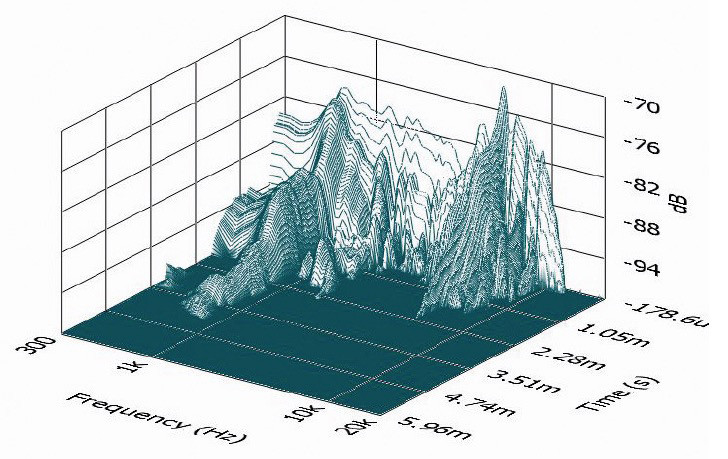
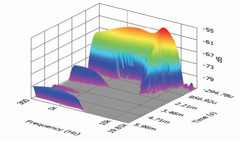
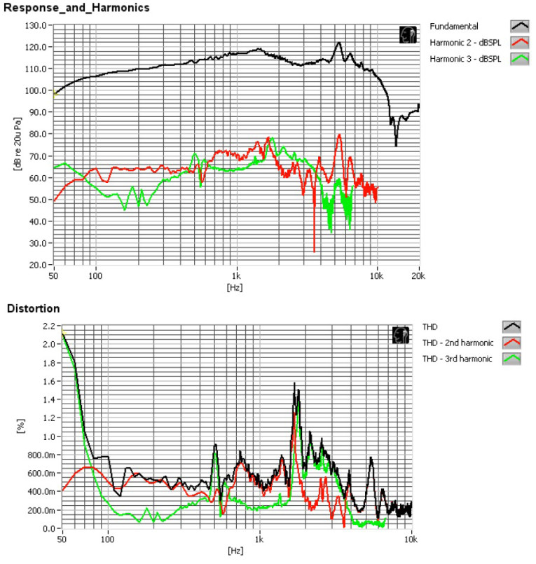
For the RS180P-8’s remaining tests, I used the Listen SoundCheck software, SoundConnext analyzer, and SCM microphone to measure distortion and generate time-frequency plots. For the distortion measurement, I mounted the RS180P-8 in free-air. I used a noise stimulus to set the SPL to 94 dB at 1 m (6.8 V). Then, I measured the distortion with the Listen microphone placed 10 cm from the phase plug. Figure 13 shows the distortion curves. I used SoundCheck to obtain a 2.83-V/1-m impulse response and imported the data into Listen’s SoundMap time/frequency software. Figure 14 shows the resulting CSD waterfall plot. Figure 15 shows the Wigner-Ville plot. For more information, visit www.daytonaudio.com. VC
This article was originally published in Voice Coil, May 2014.