Progress on Calculating Edge Effect of Acoustical Absorption

Rooms in which Reverberation Time (RT) is important often require the application of acoustical treatment such as absorptive wall panels. The most obvious way to treat a wall is to cover the entire wall, and the resulting uniform appearance pleases architects and interior designers. But many “how-to” books and articles on acoustics state that absorptive material is more effective if applied only to parts of each wall, as long as untreated patches on opposing walls are avoided, in order to prevent flutter echo. This advice implies that the same area of absorption can have more or less effect in reducing reverberation, depending upon the physical shape. Although the Sabine and other statistical RT equations do not predict such an effect, experience has shown it to occur.
 
The Edge Effect
The physical reasons behind this apparent anomaly are often lumped into the category of “edge effect” — along with the observation that equally competent test labs using identical standard procedures can measure different absorption coefficients (α) that sometimes exceed unity! This latter situation has been the cause of much speculation throughout the years, with some experts stating that any α greater than unity is erroneous. If α is indeed, as Wallace Clement Sabine stated, the fraction of sound absorbed by a surface, then by definition, it cannot exceed unity.

However, as we discussed in audioXpress' April 2016 Sound Control article, using an α of unity in the Sabine equation does not give zero RT, although if α were indeed the fraction of incident sound absorbed by a material, having an α of unity would leave no sound in the reverberant field, and thus zero RT. Therefore, we must define α as a constant of a particular material which, when obtained using the standard measurement techniques and the Sabine equation, allows prediction of RT with some accuracy, given certain known limitations. This new definition validates the possibility of α > 1, although such values of α cannot be used with computerized acoustical modeling software.

However, we are left with the questions of why the absorption of a particular block of material apparently varies with size and shape, and why different values are measured in different labs. Leo Beranek states that a properly done measurement of α is accurate for the particular piece of material measured, in the specific room and location in which the measurement is performed. While true, and perhaps comforting, this statement may create as many questions as it solves. One physical mechanism that has been proposed to explain the difference in measured α among different labs is the actual diffuseness of the sound field in the reverberation chamber used for testing. Many labs have now installed plate diffusors to improve this characteristic.

Still remaining to be explained is “edge effect”: What physical processes are involved? The answer seems to be twofold:
(1) The statistical assumptions upon which the Sabine theory is based are violated in practice. When a sound field encounters the edge of a piece of absorptive material, the acoustical impedance near the material changes, causing wave refraction, with the result that the material can appear as much as a quarter wavelength larger in each dimension than it actually is. This makes near-grazing waves strike the absorber and be partially absorbed.[1]

(2) Edge diffraction causes sound crossing an edge of an absorber to change direction. This also causes an effect similar to that of a larger area of absorption. The way this works can be understood with the aid of Huygens' Principle: Every point illuminated by a wave can be considered as a spherical-wave source. Thus when an edge is irradiated by sound, the sound beyond that edge can be calculated as a superposition of all these spherical sources. This means that we can imagine a line of spherical radiators at the edge of the absorptive material, and thus, calculate the strength of the diffracted sound in any location.

Since the radiation is spherical, sound is transmitted in all directions, including along the vertical and the horizontal surfaces of the absorber’s edge. In the case of diffraction, the amount by which the absorber’s effective area increases is proportional to the ratio of the perimeter of the edges to the area of the absorber.

α Measurements
At InterNoise 2009, Ron Sauro of NWAA Labs presented the results of measurements of RT in a test lab with absorptive material of a given area — measured first in a single piece, then cut into pieces so that the area could be held constant while the perimeter varied. 

His measurements demonstrated three things:
• α varies with both area and perimeter.
• α varies substantially with frequency, particularly above 250 Hz and for very absorptive materials.
• The measured absorption coefficients approach 1.5.

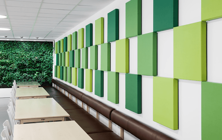
These results verify the oft-repeated advice to treat walls with patches of absorption rather than single large sheets, when the purpose of treatment is to control RT. The usual calculations for evaluating the effects of absorption, including equations and ray tracing, cannot give reliable predictions in all cases. Investigations are ongoing to determine how to better specify a material’s α and account for the effects of size and shape. Absorption coefficients are measured in a reverberant chamber. A sample of the material is placed according to internationally standardized procedures, and the reverberation time is measured. The RT in the room obeys the Sabine equation:
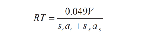
where s_c and s_s are the areas of the chamber boundaries (walls, ceiling, and floor), and of the absorptive sample, respectively, V is the volume of the chamber in cubic feet, and α_c and α_s are the sound absorption coefficients of the chamber material and of the sample. Solving for α_s and calculating the product s_c α_c from the chamber dimensions and the RT of the empty chamber, we can determine α_s from:
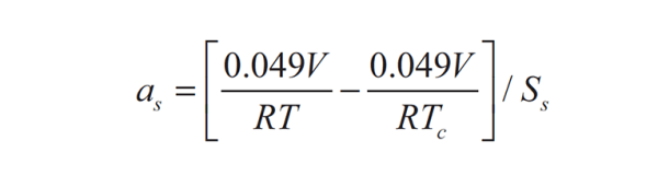
RT_c is the RT of the empty chamber.

New Theories
S-I Thomasson investigated the effect of area upon sound absorption.[2] He developed models for including the effects of absorber size and the angle of sound incidence.

As discussed in the April 2016 Sound Control article, Ron Sauro proposed an alternative to simple absorption coefficients based on making multiple measurements with different perimeter: area ratio configurations. His method accurately accounts for edge effects, but does require multiple measurements for each material.

International Standards Organization (ISO) working group TC43/SC2/WG30 has a proposal based on Thomasson’s paper. However since this proposal has not been finalized, we are unable to publish details at this time. Robert Hallman of Armstrong World Industries is also working on edge effects. He presented a paper at the April 2017 American Society of Testing and Materials (ASTM) meeting in Toronto, ON, in which he discussed a method he has developed that accounts for edge effect without requiring extra measurements. This has obvious benefits for manufacturers, who will not have to invest in re-measuring all their absorption products, and for acousticians who will not have to update their reference tables of material absorption coefficients. The method is empirically derived. Hallman’s method produces results that match the measured data for the several configurations of absorption that he tested.

Hallman’s method defines a virtual area of the absorptive material that is the sum of its actual area plus a wavelength-related area associated with the perimeter. Its goal is to provide a way to predict the absorption of various sample sizes and geometries without requiring change to the absorption coefficients. In this, it is similar to Thomasson’s method, but Thomasson used an added perimeter area corresponding to the area of material within λ/4 of the edge; whereas, Hallman added a perimeter area corresponding to a distance λ/2 from the edge. Hallman then incorporated a method to avoid adding the corners of the perimeter area twice, as occurs in Thomasson’s method. 
  Next, he calculates a total absorption for the piece of material based upon the material dimensions and the sound absorption coefficient α as measured by ASTM standard C423, the present standard for measurements. Thus, existing α values can be used. In Hallman’s presentation, he showed the total absorption in Sabins measured for each of five samples: 6’ × 6’, 8’ × 8’, 10’ × 10’, 12’ × 12’, and a 10’ × 10’ sample cut into 25 2’ × 2’ pieces and scattered, as Sauro had done with spaces between the pieces (see Photo 1). The total absorption in Sabins for each sample is plotted vs. frequency in Figure 1. Notice that, while the total absorption increases with area, there is also some frequency dependence, especially in the case of the separate 2' × 2' pieces.

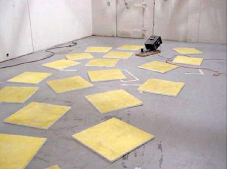
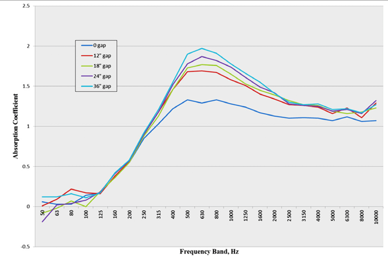
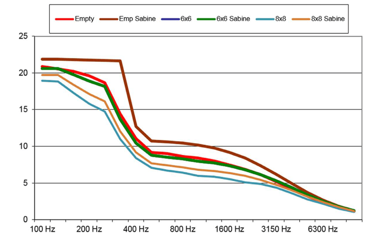
Next, Hallman showed the effects of separation between 2’ × 2’ pieces, in samples containing nine such pieces (see Figure 2). Based upon these results, he omitted the separated samples from further comparisons, focusing instead on the effect of sample area and perimeter. Although European measurements of α use a square material sample, American measurements use the 8’ × 9’ size specified in ASTM C423. (Apparently, this size is an artifact of a practice used at Riverbank Laboratories in years past.)
 
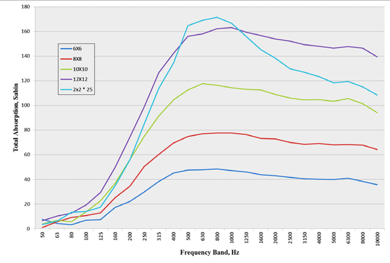
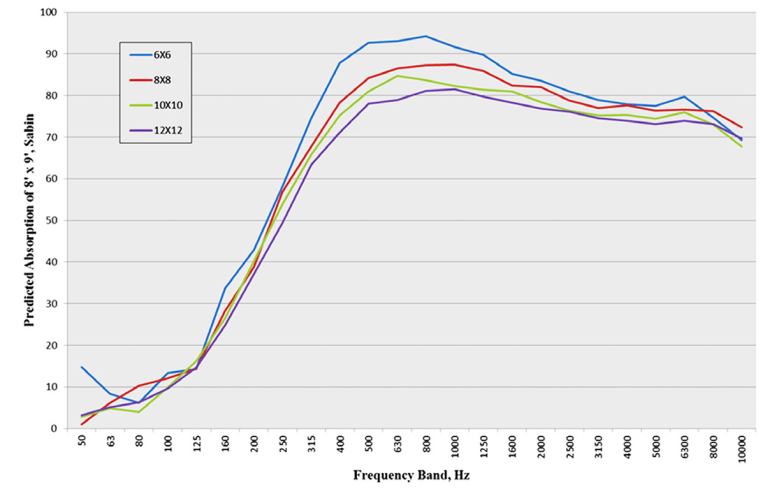
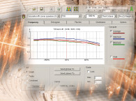
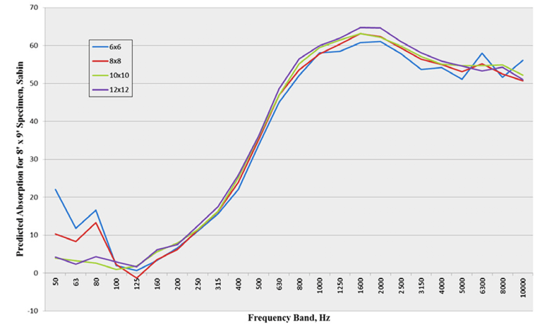
Using the measured α values for the four square samples whose absorption was compared in Figure 1, Hallman calculated the value that a standard 8’ × 9’ sample would exhibit (see Figure 3).

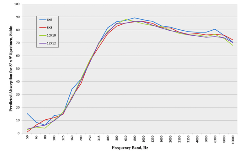
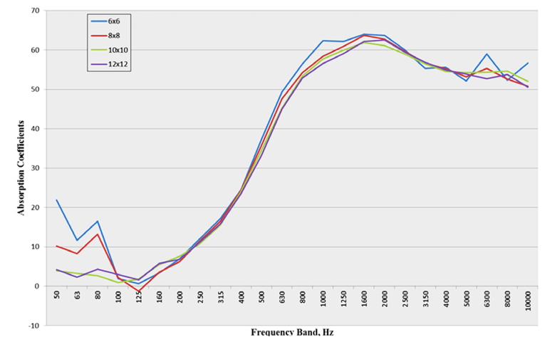
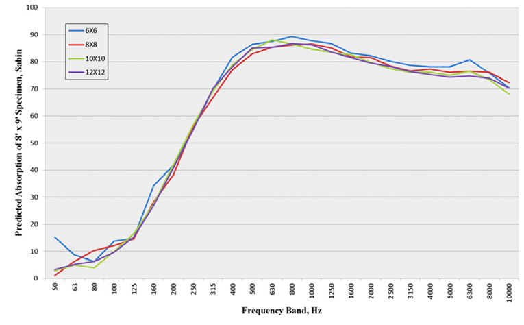
Figure 4 illustrates that applying Hallman’s method to the process used to generate Figure 3 gives good agreement among the resulting curves. These results for fiberglass panels, a highly absorptive material, were encouraging, so Hallman next tested mineral fiber panels, which are less absorptive. As shown in Figure 5, the variation in the total absorption of an 8’ × 9’ panel predicted using the α values for the 6’ × 6’, 8’ × 8’, 10’ × 10’, and 12’ × 12’ samples was less than for the high-absorption panels.

You can see from Figure 6 that Hallman’s method also showed less variation in predicted total absorption than that for the fiberglass, but seems to have over-corrected in that the absorption predicted using the α from the smaller sample is now less than that predicted using α values from larger samples. He addressed the over-correction by using a modification of α for the perimeter area.

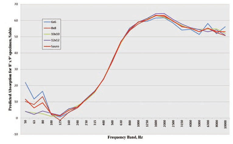
Next, Hallman compared the predictions from his revised method with those from Sauro’s method — see Figure 7 (fiberglass panels) and Figure 8 (mineral fiber panels). The two methods substantially agreed for both fiberglass and mineral fiber samples. However, more work is needed to understand the effects of separation between/among pieces of a “scattered” sample. Also, agreement between methods is poor in the 1/3-octave bands below about 160 Hz.
   
Testing the Theories
Both Sauro’s and Hallman’s methods have been assessed in terms of Sabine’s or other statistical acoustics analysis. I was curious whether ray-tracing analysis would show any difference among the absorption predicted for samples of different areas in a modeled reverberation chamber. One would not expect there to be a difference, but I decided to check it out anyway.

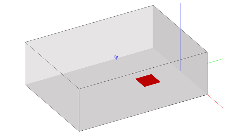
Figure 9 shows the model of the chamber with a 6’ × 6’ sample of 1″ fiberglass. I ran simulations to determine the RT for the four sample sizes used in Hallman’s tests. The RT graphs are shown in Figure 10. The Sabine-predicted RT is also graphed. As usual, there is a small difference between the Sabine and the ray-traced RT predictions, and as expected, RT is smaller with samples of larger size. But did the effective α vary among samples? Figure 11 illustrates the variation of α calculated from the chamber dimensions and volume, and predicted RT.
 
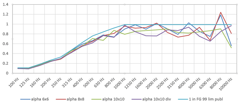
The published α of the 1″ fiberglass panel is also graphed for comparison. Due to the limitations of ray-tracing modeling programs, the maximum α has been limited to 0.99. The α derived from ray tracing follows the published values for the material within 10% or less, except at the highest frequencies.

The raggedness of the curves may be due to EASE’s limiting the precision of results to two decimal places. (In digital audio, we’d call that “quantizing noise.”) The bottom line is that when absorptive areas of dimensions other than 8’ × 9’ are used (often!), ray-trace models will have some errors in RT calculations, since they cannot take the size of absorptive areas into account. The quest for ways to accurately predict RT in a room continues! aX

This article was originally published in audioXpress, December 2017.

References
[1] Cheol-Ho Jeong, “Sabine absorption coefficients to random incidence absorption coefficients,” 
www.sengpielaudio.com/AbsorptionsgradGroesserEins.pdf

[2] S-I Thomasson, “Theory and Experiments on the Sound Absorption as a Function of Area,” Report TRITA-TAK 8201, Royal
Institute of Technology, Sweden, 1982.