Some people have attempted to come up with creative solutions to obtain the free-field response of a speaker, such as driving their test gear to the middle of a large parking lot or suspending a speaker from their child’s zip line. However, there is a simpler solution — a “splice” measurement. This is a long-established technique — I wrote an Audio Engineering Society (AES) paper on the subject back in 1992, and the capability for such measurements has been included in SoundCheck since 2001. Despite its long history, this method has not seen widespread use. However, the current pandemic’s working challenges are sparking renewed interest.
Free-field measurements contain only direct sound propagation, with no sound reaching the ear (or microphone) from reflections. Such measurements are usually made in anechoic chambers as the usual alternative—a very large open space high enough above the ground to avoid reflections—is impractical. While accurate near-field measurements can be made in a regular room at low frequencies, they do not represent the free-field response at higher frequencies. Far-field measurements are inaccurate when made in regular rooms as they are always subject to reflections that interfere with the measurement. These can be windowed out using a Log TSR signal and time-windowing, but at low frequencies, the room size limits the width of the time window and, therefore, the corresponding frequency resolution.
It should also be noted that all anechoic chambers have a low-frequency cut-off due to their size; the larger the chamber, the lower the frequency that you can accurately measure down to. This means that in many cases, an anechoic measurement may not be particularly accurate at low frequencies, especially if the chamber is small.
Accurate free-field measurements can be obtained in a regular room without an anechoic chamber by making what is known as a “splice measurement.” This consists of a near-field measurement covering the lower frequencies, and a time-windowed far-field measurement, joined together in the range where both measurements are still valid and overlap. A complete mathematical explanation of the validity of this method can be found in the 1992 AES paper titled ‘‘Simulated Free Field Measurements” that I co-authored with Christopher J. Struck. This principal could, of course, be realized with any measurement system, although implementation can be complex.
Practical Test Sequence
The measurement is significantly simplified with a SoundCheck test sequence that walks the operator through the measurement and splicing process, complete with prompts advising what to measure and how to splice the sequence together. Originally written 10 years ago, this test sequence has recently been updated to offer flexibility for both ported and unported speakers. Ported speakers require the addition of a second near-field measurement at the port location that is added into the combined response.
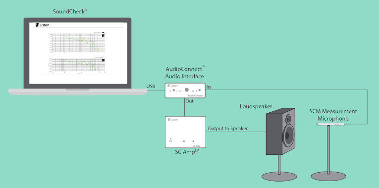
All that is needed for making such measurements is SoundCheck 18 (or newer) with the optional LogTSR stimulus module (this can be added to any current system), plus a microphone with appropriate power and audio interface. The test configuration shown in Figure 1 includes the compact AudioConnect test interface, which contains audio in/out, as well as the microphone power supply. An optional amplifier is added if the speaker requires power. An SCM measurement microphone completes the setup. Alternative audio interfaces, amplifiers, and microphones may, of course, be used.
When starting the sequence, the user is asked whether or not the speaker is ported. The user is then advised to place the microphone very close to the low-frequency driver (less than 1”) and the near-field frequency response is measured using a 1/12 octave stepped sine. If the speaker is ported, the measurement must be repeated at the port.
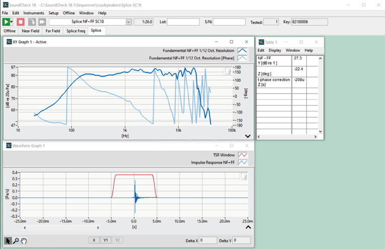
Next, the user is prompted to place the microphone in the far field, and the frequency response is measured using a continuous log sweep with the Time Selective Response analysis algorithm. A graph shows the initial signal, plus reflections, and a suggestion made for where to window the signal (see Figure 2). This suggestion is based on the first strong reflection, and everything after this in the time domain is removed. The window may be user-adjusted based on what is seen on the graph.
The two graphs are then displayed together, and the user selects the splice point based on the overlap in shape of the two graphs. Although there is a little subjectivity here, it is usually fairly obvious, and the precise point on the curve is not critical as long as it is within the overlapping range. Once the splice point is selected, the two curves are stitched together to give the speaker’s complete frequency response. This is done in several post-processing steps including the inverse fast Fourier transform (FFT) of the final frequency response back to the time domain to calculate the impulse response for the loudspeaker’s entire frequency range. Differences in amplitude and phase are automatically corrected. The final display shows the spliced frequency response and phase measurements, as well as the time window used, and the phase and amplitude corrections applied.
The sequence can be run with stored data, and experimentation with the time window can be performed without having to re-measure data. The curve data and time waveforms (e.g., impulse response) can also be analyzed in SoundMap, SoundCheck’s time-frequency analysis module, or exported for further analysis. As with all of Listen’s test sequences, this sequence can be user-modified. For example, distortion analysis could be added.

Practical Demonstration and Example Results
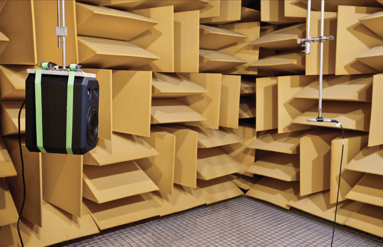
Indy Acoustic Research, an independent audio consultancy, measured the same speaker, a Tannoy System 600 two-way co-axial speaker, in its anechoic chamber and used the splice sequence in its laboratory to compare results. First, measurements were made in an anechoic chamber using a conventional stepped sine sweep to show the true anechoic response (Photo 1). The speaker was suspended in the chamber, and the 1/2” free-field microphone was positioned at 1m on-axis.
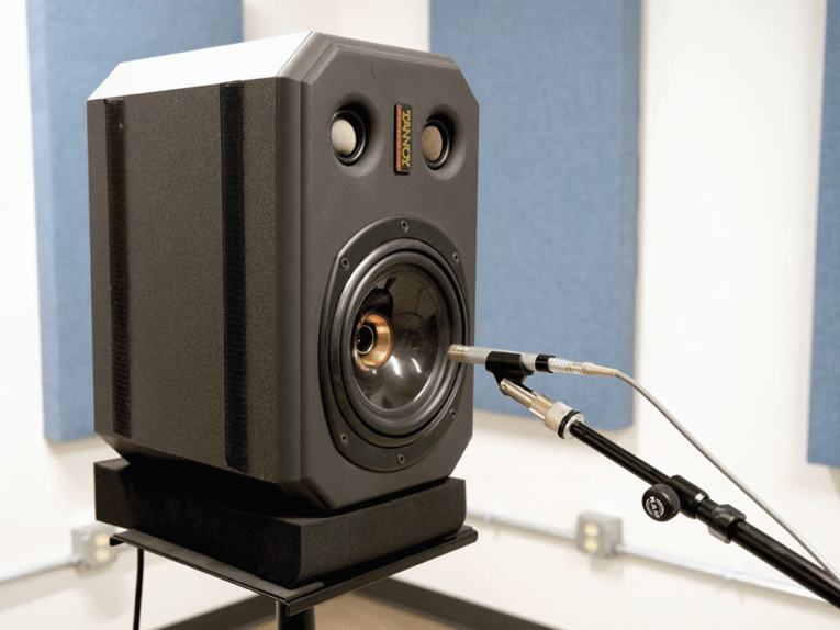
Next the same speaker was measured in the laboratory (Photo 2 and Photo 3). The 19.5’ × 12.5’ × 9’ room includes drywalls and ceiling, a vinyl floor with carpet, and some acoustic treatments on the walls. In other words, it is a fairly typical room with many reflective surfaces.
The speaker was mounted on a stand away from the wall. The microphone was placed at 1m on-axis for the far-field measurements, and 5cm on-axis for the near-field measurements, Care was taken to ensure that the far-field microphone positioning was the same as for the anechoic chamber measurement.
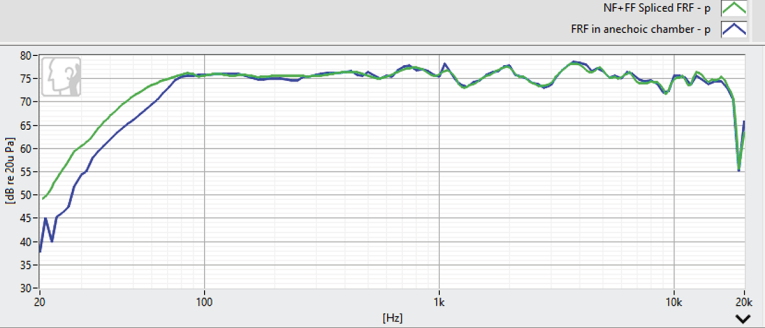
Figure 3 shows both the anechoic and the splice sequence results. The correlation is clear, particularly above 100Hz where the results are almost identical. The discrepancy in the lower frequency range is to be expected, since the acoustic chamber is small, measuring approximately 3m × 3.7m × 2.6m, and it has a cut-off frequency of about 120Hz.
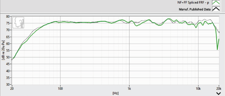
The simulated free-field measurement was also compared to the manufacturer’s specifications by overlaying the published curve onto the measurements as seen in Figure 4. Here, a much closer correlation in the low frequencies is observed. This is likely because the manufacturer’s measurements were made in a much larger chamber with a lower cutoff frequency and, therefore, closer to a true anechoic response. At higher frequencies, you can see that the curves are very close and essentially the same shape; the slight variations can be attributed to microphone positioning. It is expected that if the exact same positioning used as in the manufacturer’s specifications had been replicated, identical results would have been obtained.
These results demonstrate how simulated free-field measurement using a splice sequence to combine near-field measurements and time-windowed far-field measurements yield results that align well with those made in an anechoic chamber. Indeed, this method is likely to yield even more accurate results at lower frequencies due to the limited size of many chambers. This technique is of value to anyone seeking to make anechoic speaker measurements without investing in a costly chamber, or seeking to make free-field response measurements while working from home. VC
Resource
C. J. Struck and S. F. Temme, “Simulated Free Field Measurements,” presented at the 93rd Audio Engineering Society (AES) Convention, San Francisco, CA, 1992.
https://content.listeninc.com/sff-measurements
This article was originally published in Voice Coil, March 2021