A fairly obvious implication of this is the significant velocity associated with the air flow through the port. This, in turn, causes all sorts of non-musical noises to be generated by the port, as well as distortion and acoustic compression. Depending on port geometry and required low-frequency SPL of the system, the issue can be quite significant.
The problem just described belongs to a rather complex field of fluid flow theory. Assuming incompressible flow, some sophisticated FEM programs would be able to model air turbulence and associated vortex shedding in more detail(1), but this is well beyond the scope of this article. Fortunately, existing research results, design material, and test results enable us to formulate an approximate macro view of the problem and look at the acoustic impedance of the port under high air velocity. I would like to stress that the approach I am taking here is a significant simplification of the physics of the problem. However, the resulting model is quite useful and is confirmed in practical tests(2).
Intuitive Approach to Port Nonlinearity
You are no doubt familiar with the need for good carpentry skills when building speaker boxes. Accuracy of joints and sealing the box is essential for proper operation of all types of boxes, be they sealed, vented, passive radiators, and so on. A sealed box means exactly that — the air inside the box is trapped and sealed from the external world. There is no parasitic or accidental leakage from the box, so that the mathematical model developed for the enclosure continues to be accurate. Consequently, the box QB factor is controlled by the designer and not by sloppy workmanship.
A vented enclosure also needs to be “air tight”; of course, with the exception of the purposefully introduced opening port. Just as for the sealed box, the cabinet needs to be sealed, so that no accidental air leakage from the box can occur. A properly executed design would include all sorts of seals and gaskets to ensure that connector boards or drivers themselves do not cause air leakage.
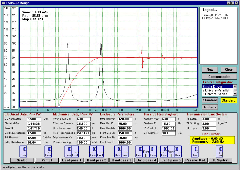
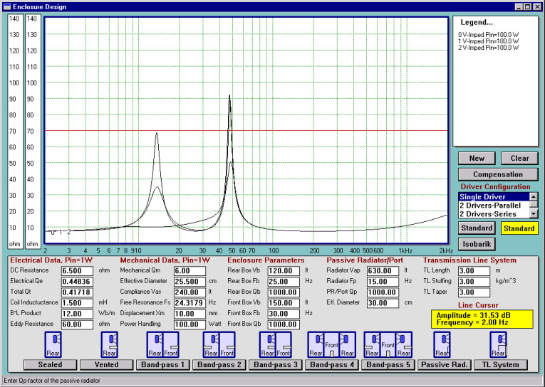
Assuming you have built your perfect vented box, you may expect that the SPL curve and input impedance curve will look as in Fig. 1. The impedance curve is very familiar and has two characteristic peaks with the dip between them. The dip is located exactly on the box tuning frequency, fB = 25Hz. My design is a QB3 type with system parameters as shown on Fig. 1, and I have also assumed that QB = QP = 1000, so I have a very low-loss design. Port diameter in this example is 15cm (6″) and the input power to the system is 1W.
Now, assume that I start reducing port diameter. Initially, the picture will not change much. However, when the port eventually becomes very small, intuitively there should be very little difference between the vented box with a “very small port” and the sealed box with a “large leakage” problem(3).
In this case, you would expect the SPL curve will resemble that of a leaky sealed box and the input impedance curve will lose the lower peak and become a “single peak” curve just like those of the sealed boxes. Between those two extremes, you may expect problems commonly known as “port nonlinearity.”
Historical Research on Fluids in Tubes
Bies and Wilson(4) actually experimented with an orifice (more like a decent port) 9cm (3.5″) in diameter and 2.9cm (1.13″) long. They found that the acoustic resistance, R, of the tube varies with the particle velocity in a similar way as shown in Fig. 2. Thurston(5), working with fluid flow through circular tubes, found that analogous acoustic resistance, R, and inductance, M, again vary in a similar way as shown in Fig. 2.
A landmark paper by Ingard(6) offers an empirical formula for the nonlinear component of the acoustic resistance of a tube. Later on, this work was expanded by Ingard and Ising(7), who offered more complete mathematical treatment of orifice behavior.
Backman(2), experimenting with port nonlinearity, plotted drivers’ input impedance for various input voltages and determined that the most sensitive to the amplitude variations is the magnitude of lower impedance peak. He pointed out that the behavior of the vented enclosure approaches a sealed enclosure at high levels. The inner diameter of the port was 102mm (≈4″), and the length of the port was 168mm (≈6.6″).
Vanderkooy(8) measured and analyzed port performance at high levels and proposed a simplified nonlinear model of a port. The comprehensive analysis included jet formation, acoustic compression, turbulence noise, and distortion.
Simplified View of the Problem
Typically, the area of the cone is many times larger than the area of the port. Since the volume of the air pushed via the port needs to be approximately equal to the volume displacement of the cone, the only way to accomplish this is to push the air in the port much faster. At low SPL levels, the volume displacement of the cone is small, and, consequently, the cone velocity is low as well. This, in turn, stipulates low air velocity in the port, or what is known as a laminar air flow.
The process is characterized by a low Reynolds number, Re<2000, and there is no turbulence in the air flow.
Re = (r × Vmax × ρ)/μ
where Vmax is the peak flow rate, ρ is the density, μ is the air viscosity, and r is the port radius. At this point, the acoustic resistance of the port, RP (port loss), is linear and is relatively low (50–200Ω).
Also, the mass of air in the port, MP, is constant. Remember that mass of the air in the port resonates at fB (box tuning frequency) with the compliance of the air inside the box halting the movement of the cone. If there were no losses, at resonance, fB, all acoustic output of the system would come from the port.
Now, start reducing the port diameter. As you can guess, the volume displacement of the cone remains the same, so the air in the port must move faster and faster. Soon, a turbulence occurs in the air flow, jets of air are forming, and the process is no longer linear. The Reynolds number corresponding to the onset of turbulence is Re ≈ 20000.
When the Reynolds number hits 50000, your vent is compressing. It is now more and more difficult to push the air in the vent. The acoustic output of the port is below the expected level (if the process continues to be linear), and you begin to experience a “port compression” effect.
Port impedance, Zp, now has an additional component relating to turbulent air flow and depending on the air velocity, RP(v). Also, the MP has changed as well, drifting towards 60–70% of its original value and becoming velocity dependent.
The RP(v) is an interesting element. If plotted in the frequency domain, it would resemble the curve depicting port air velocity (Fig. 3). This should be no surprise, as RP(v) is so heavily dependent on the port air velocity. In the frequency domain, the RP(v) will quickly reach its peak not far from the lower peak of the input impedance curve. Depending on the geometry of the port and the volume displacement of the driver, the air velocity in the port may reach 50–100m/s. Such a high value of air flow results in RP(v) reaching 5–10kΩ levels.
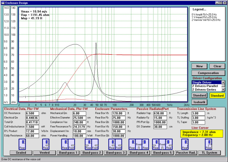
The “double-peak” impedance curve is a clear result of the port action. The port air velocity curve plotted on Fig. 3 clearly indicates that the lower impedance peak will be much more affected by the port nonlinearity than the upper impedance peak. Therefore, the RP(v) needs to be incorporated in the driver’s model.
Changes in Driver’s Model
The vented enclosure shown in Fig. 4 provides different loading for the back of the diaphragm, as compared to the sealed box. The vibrating system and front loading of the diaphragm are represented on the mechanical mobility circuit the same way as for the sealed enclosure.
Introduction of the vent adds several more components such as: (1) mass of the air in the port (Mmp) and its losses (Rmp), and (2) radiation impedance of the port represented by Rmrp and Mmrp. The air in the port is treated as a mass because of its small volume and, more important, because it is incompressible. Particles of air will move on both sides of the vent with the same velocity. The air compressed in the box by the back side of the diaphragm has only one path for escape — pushing the air mass through the vent. Therefore, the pressure path consists of the series connection of Cmb, representing compliant air in the box and the four elements of the port.
Since the air in the port is incompressible, the immediate layer of air in front of the box (radiation impedance) will be connected to the same velocity line as the entry to the port inside the box. The other end of the masses is connected to the U = 0, or reference velocity as required in mechanical mobility circuits.
The mechanics of the preceding process can be easily demonstrated on a physical model of a vented box. Connecting a small (1.5V) battery across vented box terminals, you can displace the cone in or out of the box. A small air-flow detecting device (candle) positioned in front of the port will show significant air movements in the direction opposite to the diaphragm.
The volume of air displaced by the cone should be similar to the volume of air leaving the port. If the difference is significant, then leakage losses are significant. This experiment clearly shows the pressure (current) path in the mechanical mobility model, so it should now be easy to explain why the compliance of the box is connected in-series with port elements. It is observable that Cmb and Mmp+Mmrp form a series-resonant circuit in the mechanical mobility representation.
The circuit will act as a “selective short circuit” for the volume velocity Uc, shorting it to U = 0 (ground) at the circuit resonant frequency. Because of the circuit losses, the short is not perfect, but velocity Uc will be much reduced. In the practical system this situation translates into much reduced cone excursion at the box resonant frequency.
Acoustical impedance representation shows CAS and Map+Marp forming a parallel resonant circuit. Electrical circuit theory advocates that very little energy (current) needs to be fed into the circuit for it to resonate and for the current (volume velocity) in the resonant circuit to be still very high.
Therefore, volume velocity in the “feeding” branch, which contains diaphragm output, will be very small, and volume velocity in the resonant circuit containing port will be high. This effect, although the strongest on the resonant frequency fB, will extend over some narrow frequency range, and on the low end side produces extended system output.
The enclosure/port resonance effect is being exploited here to augment system output at low frequency. Figure 4 shows mechanical mobility (top diagram) and acoustical impedance (bottom diagram) representation adopted for the vented enclosure model. The components are:
• CAS, equivalent compliance volume VAS transformed to acoustical side.
• Mad, mass of the vibrating system Mms transformed to acoustical side.
• Ras, vibrating assembly loss Rms transformed to acoustical side.
• Mar+Mab, air radiation of the front side of the diaphragm and air load of the back side of the diaphragm.
• Rar, air radiation of the front side of the diaphragm.
• CAB, enclosure compliance VAB transformed to acoustical side.
• Rab, absorption losses of the enclosure transformed to acoustical side.
• Marp, Rarp port radiation.
• Map, mass of the air in the port.
• Rap, frictional losses in the port.
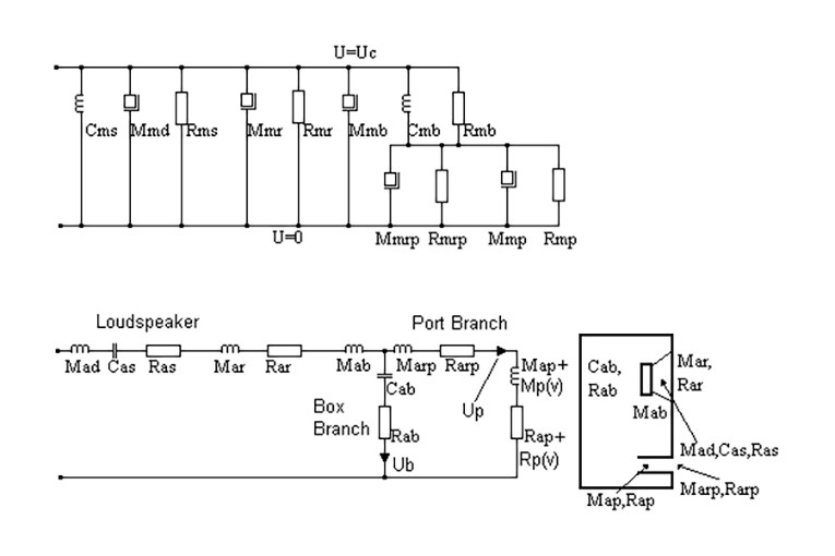
The nonlinear port impedance was implemented as Zp(v) = RP(v) + jωMP(v) in the port branch. Please note that Map+MP(v) will exhibit a slight reduction in value as the air speed increases, and Rap+RP(v) will exhibit significant increase in value as the air velocity in the port increases.
Resulting Performance
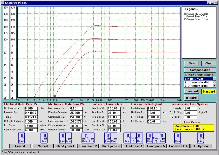
In order to gain some insight into system performance affected by port nonlinearity problems, I plotted the SPL for a port of 5cm in diameter for 1W (curve 0), 10W (curve 1), and 100W (curve 2) input power (Fig. 5). As you can see, with the increased input power, there is a sort of “saddle” developing on the SPL curve around the box tuning frequency of 25–30Hz. This is exactly the frequency range where you would expect the port to contribute most to the system SPL. Our small port is clearly not performing as anticipated.
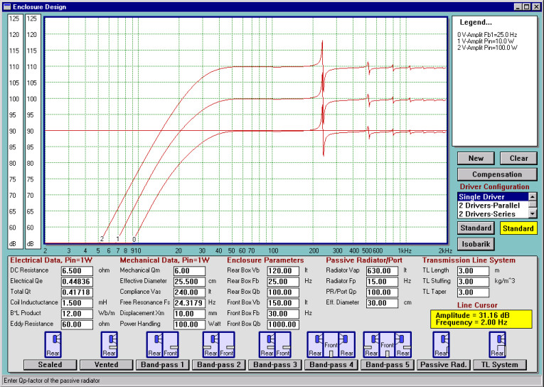
Next, I modeled SPL for the same power levels, but this time I used a larger port, 15cm in diameter. The resulting plots in Fig. 6 do not exhibit the “saddle” any more for the 100W power level. Clearly, as the input power is increased, the SPL curves go up, maintaining the approximate shape acquired at 1W power level.
It is also easy to observe that the SPL curves now have resonant peaks above 200Hz, not seen in Fig. 5. This is the result of enlarging the diameter of the port. You may remember that larger port must also be longer if tuned to the same frequency. The length of the port is such that the self-resonances of the port tube fall into a much lower frequency range — just to be displayed on the screen.
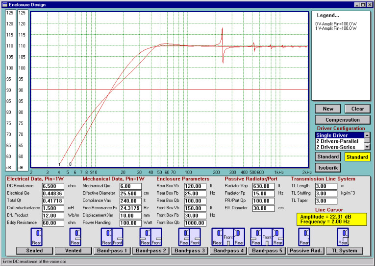
In order to estimate “port compression” effect, I plotted the SPL of the two ports on the same screen (Fig. 7). Visual inspection of the graphs shows about 5dB of port compression at fB = 25Hz. I have just about lost my vented box performance gains if I were to use the smaller port.
In the next step, it would be interesting to compare the input impedance plots to see whether the lower impedance peak, characteristic for the vented enclosure, indeed disappeared from the plots. The answer is clearly evident in Fig. 8, where the input impedance for three ports is plotted at 100W power level. The 15cm vent exhibits the expected “double peaks” curve; however, the compression is still registered on the impedance plot. Ideally, the port should still be larger.
The Reynolds number calculated for these conditions is Re = 68000. Therefore, the port is indeed compressing slightly. However, the 10cm port has the lower impedance peak significantly reduced. This is a sure sign that this port is too small for the job. The severely undersized 5cm port produces a “single peak” impedance curve for 100W input power. This port would also prove to be inadequate for 1W of input power. The Reynolds number calculated for 1W conditions is Re = 20000, which is a clear indication that the port becomes turbulent.
Indeed, the corresponding input impedance plot shown in Fig. 9 is a clear indication of the nonlinearity problem at 1W for this port.
Remedies
First and foremost, the problem is related to air velocity in the port. As we know(9), air velocity in the port, Vp, depends on volume velocity Up via the port branch divided by the port’s area, Sp.
Vp = Up/Sp
Since the area Sp = πr2, it is easy to observe that air velocity in the port depends on the inverse squared of the port’s radius. It seems rather obvious that port radius should be kept as large as possible.
Dickason(10) recommends 15cm (6″) ports for 15″ woofers as a minimum and 10cm (4″) ports as a minimum for 12″ woofers. Salvatti(3) offers a number of recommendations relating to port geometry, including balancing inlet and exit flows by using different tapers. Roozen(1) advocates port geometry based on 6° diverging contour towards the ends of the port. The inlet and outlet are rounded with a relatively small curvature.

Conclusions
I have described a simple modification of the acoustic impedance of the port in the vented enclosure. The modification consists of adding extra components such as MP(v) and RP(v), which are dependent on air velocity inside the port.
The modification reflects acoustic compression of the port and shows the changes to the input impedance of the driver under high SPL levels. The changes in input impedance reflect experimental findings(2).
Looking at the performance of the 15cm (6″) vent, I was surprised to see the compression evident at 100W input power. The vent seems quite large, and to tune it to 25Hz in a 120 ltr box, I would need to make it nearly 60cm (23.6″) long. This could be a construction challenge, and besides, this vent is still not completely linear at high SPL. This brief analysis of the vent performance clearly indicates that nearly all practical size vents will compress at higher SPL levels.
Loudspeakers intended for high power stage applications should give very careful consideration regarding port nonlinearity. For this type of application, the port compression problem will tend to further degrade system SPL, already affected by the thermal compression during prolonged stage performance. aX
References
1. N.B. Roozen, J.E.M. Veal, J.A.M. Nieuwendijk, “Reduction of Bass-Reflex Port Nonlinearities by Optimizing the Port Geometry,” AES preprint 4661.
2. J. Backman, “The Nonlinear Behavior of Reflex Ports,” AES preprint 3999.
3. A. Salvatti, D. Button, A. Devantier, “Maximizing Performance from Loudspeaker Ports,” AES preprint 4855.
4. D. Bies, O. Wilson, “Acoustic Impedance of a Helmholtz Resonator at Very High Amplitude,” JASA, Volume 29, Number 6, 1957.
5. G. Thurston, “Periodic Fluid Flow Through Circular Tubes,” JASA, Volume 24, Number 6, 1952.
6. U. Ingard, “On the Theory and Design of Acoustic Resonators,” JASA, Volume 25, Number 6, 1953.
7. U. Ingard, H. Ising, “Acoustic Nonlinearity of an Orifice,” JASA, Volume 42, Number 1, 1967.
8. J. Vanderkooy, “Nonlinearities in Loudspeaker Ports,” AES preprint 4748.
9. R. Small, “Direct Radiator Loudspeaker Analysis,” An Anthology of Articles on Loudspeakers from JAES Vol. 1–Vol. 25 (1953–1977).
10. V. Dickason, Loudspeaker Design Cookbook, 7th Edition - https://cc-webshop.com/collections/books-audio/products/loudspeaker-design-cookbook
11. G. Thurston and others, “Nonlinear Properties of Circular Orifices,” JASA, Volume 29, Number 9, 1957.
12. 12. A. Nolle, “Small-Signal Impedance of Short Tubes,” JASA, Volume 25, Number 1, 1953.
13. G. Thurston, C. Martin, “Periodic Flow Through Circular Orifices,” JASA, Volume 25, Number 1, 1953.
This article was originally published in audioXpress, September 2001.
About The Author
Bohdan Raczynski has a masters degree in Acoustics and is currently a director of software company, Bodzio Software, in Melbourne, Australia. Born in Poland, he developed a passion for audio and electronics in his teens. After graduating from Polytechnik of Gdansk in Poland, he designed a number of valve and solid-state power and high power amplifiers. He moved to Australia and in 1990, developed his first commercial program, Speaker System Designer (SSD), which became available first in Australia and then US and Europe. In mid ’90, he replaced SSD with the now well-recognized SoundEasy. Bohdan lives in the eastern suburbs of Melbourne with his wife and three children.