When performing electroacoustical response measurements, an important practical consideration is the reduction of uncorrelated background noise.
Synchronous averaging (i.e., “complex averaging,” “time domain averaging,” or “vector averaging”) is a technique originally developed to analyze the vibration signature or rotating machines and gearboxes. It can be used to improve the S/N ratio measurement.
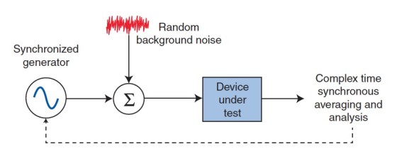
In a loudspeaker test, a correlated test stimulus, which is identical for every record, adds on a “Signal” basis (i.e., 2x = X + 6 dB), while the uncorrelated background noise, which is the same level (but not the same signal), adds on a power basis (i.e., 2x2 = X + 3 dB).
In Figure 1 all samples are treated as complex vectors (i.e., magnitude and phase), rather than simple power averaging. Therefore, an effective measurement S/N increase of 3 dB is gained for every doubling of either the measurement time or the number of complex averages. Most analysis systems and time-selective techniques offer this option. The stimulus may be a sinusoid or a pseudo-random noise signal (i.e., a repetitive random noise with a period equal to the analysis record length).
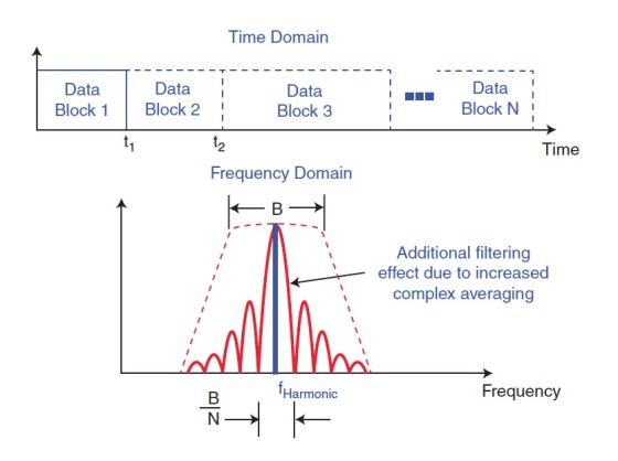
Since the averaging is complex and correlated, increasing the number of averages (i.e., sweep time) effectively lengthens the time window. Seen in the frequency domain, this is a narrowing of the main lobe of the Fourier transform of the time window, a sin(x)/x function. This can also be viewed as a more selective filter, thus reducing noise at all other frequencies. This is the effective bandwidth of the analysis, as shown in the diagram, where B is the initial filter bandwidth for the analysis (see Figure 2).
Note that for a 3-dB increase, the length of each data progressively doubles. So, the price to pay for a 3-dB improvement in measurement S/N is a geometrically increasing measurement time (i.e., two averages or double the sweep time; four averages or quadruple the sweep time; eight averages or 8 × sweep time; 16 averages; etc.). Note also that since the stimulus is synchronized to the analysis record and is zero at the beginning and end of each data block, no time window is required.
For a white background noise spectrum, the approximate amount of additional noise reduction can be computed as 20 log10√N where N is the number of averages.
About the Author
Christopher J. Struck is CEO and chief scientist of CJS Labs, a consulting firm in San Francisco, CA, specializing in audio and electro-acoustics. His areas of expertise include transducers, acoustics, system design, instrumentation, measurement and analysis techniques, hearing science, telephonometry, speech intelligibility, technology strategy, and training services.
Prior to founding CJS Labs, Christopher held positions at Brüel & Kjær, Dolby, and Tymphany. He is an Acoustical Society of America member, a senior member of the Institute of Electrical and Electronics Engineers, and an Audio Engineering Society fellow. Currently, he is the chairman and an Individual Accredited Expert of the American National Standards Institute/Acoustical Society of America Subcommittee 3, responsible for standards development in bioacoustics and related fields.