By Charlie Hughes, Excelsior Audio
Design & Services, LLC

The specification of a loudspeaker’s sensitivity is probably one of the most common, yet perhaps one of the most misunderstood. In the past, and still today, it is common to see the magnitude response of a loudspeaker system reduced to a single number as a sensitivity rating. This is perhaps at the heart of the confusion. You would think that this metric should give some indication as to how loud a particular loudspeaker will be when reproducing a signal.
You may also think that two loudspeakers with the same sensitivity rating will be equally loud when reproducing the same signal.
Each of these assertions is only partially true. A loudspeaker’s sensitivity can give an indication of its output level, but only for a signal with a specific bandwidth and spectral content. Similarly, two loudspeakers with the same sensitivity may not output the same SPL when excited by the same signal if the frequency response limits of the two loudspeakers are different.
Look at the underlying cause of each of these effects, bandwidth, and the role it plays. And also consider why sensitivity may no longer need to be referenced to a watt. According to the standard IEC60268-5, a loudspeaker’s sensitivity is determined by measuring its output when driven by a band-limited pink noise signal with a Vrms equal to the square root of the loudspeaker’s rated impedance and referencing this SPL to a distance of 1m. The bandwidth of the pink noise is limited as a function of the effective frequency range of the DUT (Device Under Test).
This is done to ensure that the test signal is confined to a portion of the frequency spectrum in which the DUT has appreciable output.
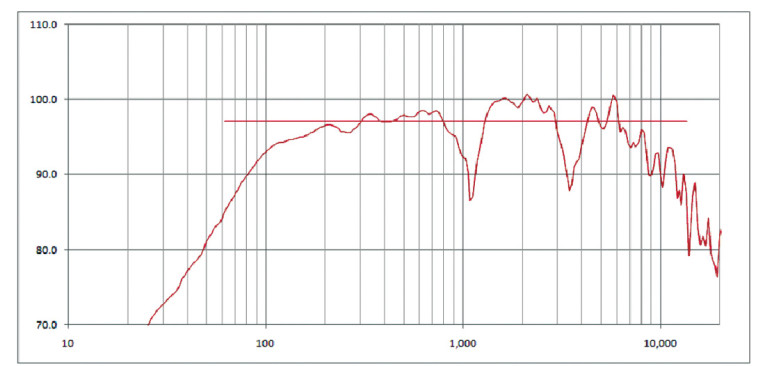
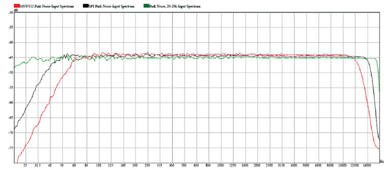
As an example, look at Fig. 1. Here you see the on-axis response of a loudspeaker. Its sensitivity rating is shown as the straight line. The length of this line coincides with the upper and lower frequency limits of the pink noise used to measure the sensitivity rating. The spectral content of this noise signal is shown in Fig. 2.
If a signal with different spectral content, but the same broadband level, were used to drive this loudspeaker, would it result in the same SPL as the sensitivity? It’s impossible to determine this without knowing both the spectral content of the signal and the response of the loudspeaker. (Note that 20Hz to 20kHz, or, in the case of Fig. 1, 110Hz–8.3kHz, does not specify the response of a loudspeaker. You need a graph of the response curve.) With knowledge of these, you can certainly make an estimate to answer this question.

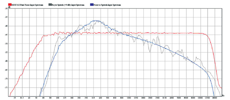
Comparing this to the response of the loudspeaker in Fig. 1, you see that the loudspeaker has limited output below 150Hz. The greatest output in the response of the loudspeaker occurs in the 300Hz–3kHz region. If the speech-shaped noise signal were used to drive the loudspeaker with the same broadband level as the noise, you could reasonably expect the broadband SPL to be greater than when driven with the pink noise signal. This is exactly what happens.
The sensitivity of the loudspeaker is 97.1dB. When driven with the speech-shaped noise, the SPL is 98.1dB, an increase of 1dB. This results from the higher level of the speech-shaped signal in the frequency region where the loudspeaker has higher output capability compared to the rest of its passband.
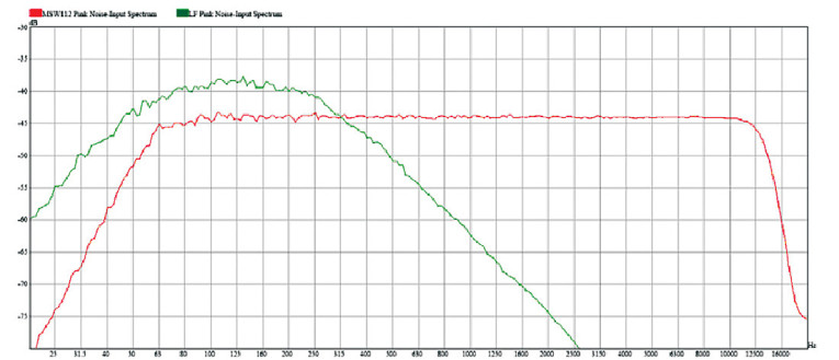
Now, compare two different loudspeakers. Figure 5 shows loudspeaker A compared to loudspeaker B. Notice that they both have the same sensitivity, 97.1dB. Loudspeaker B, however, has greater low-frequency and high-frequency extension than loudspeaker A. Because of this, the bandwidth of the pink noise used to determine the sensitivity of loudspeaker B is greater than the bandwidth of the noise used for loudspeaker A (Fig. 6). As a result, the mid-band level of the noise for loudspeaker B is slightly less than that of the noise used for loudspeaker A.
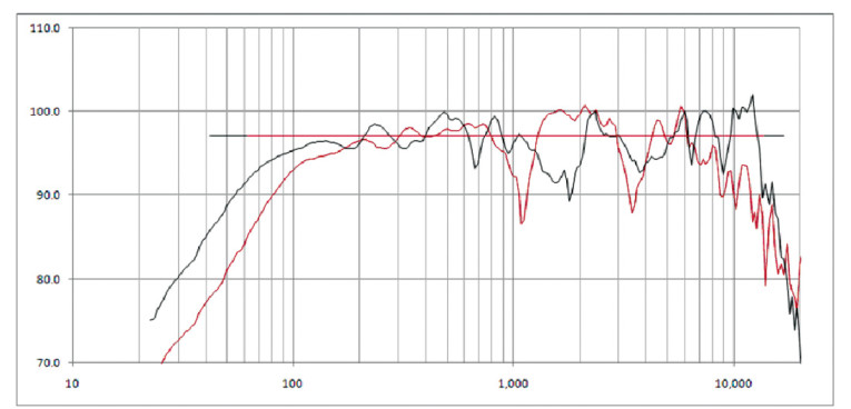
Because each of the loudspeakers used in this example is markedly not flat in its mid-band response, there may be some tonal, and potentially measurable, differences in the SPL. I hope you can put these issues aside for the moment. All other things being equal, the loudspeaker with the greater effective frequency range (low- and high-frequency extension) should have greater SPL output. Loudspeaker B should have slightly greater output when driven by this broadband pink noise signal. In fact, loudspeaker B measured 0.8dB greater than loudspeaker A, 97dB compared to 96.2dB.
From these examples you should be able to see that the SPL generated by a loudspeaker is a function of both the loudspeaker’s transfer function and the spectrum of the signal being reproduced. Several acoustical room modeling programs take this into account when calculating the SPL produced over an intended audience area. They may allow for the selection of pink noise, some sort of speech spectrum, or a user-defined spectrum. This should aid the sound system designer, while still at the drawing board stage, to better understand the potential SPL capabilities of the sound system with the typical program material the system is likely to be reproducing.
You can simplify this measurement procedure so that you don’t concern yourself with the dissipation of a real watt by the DUT. Instead you apply a voltage across the DUT that would dissipate 1W in a pure resistance having the value of the rated impedance of the DUT. This certainly is easier, but again, does this give useful information for the design and/or specification of loudspeakers or sound systems? The answer is perhaps. But I think that more useful comparative information would be gained by applying the same voltage across the DUT regardless of its impedance.
The majority of amplifiers used in sound systems today are of a constant voltage type. That is to say, their output voltage remains constant independent of the load placed on them. Of course, the load must be within the specified operational limits for a given amplifier. The salient point is that for a given drive voltage, a lower impedance loudspeaker will have greater SPL output than a higher impedance loudspeaker; all other items being equal.
Shouldn’t this be reflected in the sensitivity specification of the loudspeaker? Why, then, would you choose to use a 2V RMS signal to drive a 4Ω loudspeaker and a 2.83V RMS signal to drive an 8Ω loudspeaker to determine their respective sensitivities?
Think about it this way. Connect two virtually identical loudspeakers to an A/B selector switch driven by the same amplifier. The only difference between these loudspeakers is that one is half the impedance (rated at 4Ω) than the other (rated at 8Ω). When switching between these two loudspeakers, the output voltage of the amplifier does not change; however, the current drawn from the amplifier does. This results in the loudspeaker with the lower rated impedance producing greater SPL. Measuring and specifying sensitivity with the same voltage, regardless of the impedance of the DUT, would accurately reveal the SPL differences that occur.
I hope this brief discussion of sensitivity has shed some light on this specification and how it may translate to the real-world performance of a loudspeaker system. From these examples I hope that it is clear that the input signal and the magnitude (frequency) response of a loudspeaker will determine the SPL generated, not just the sensitivity rating of the loudspeaker. It’s much better to have knowledge of the loudspeaker’s response in the form of a graph than a single sensitivity number. The latter may be derived from the former.
Originally published by Voice Coil, April 2010