I have correct in quotes above because for a given magnitude response there are an infinite number of equally valid phase responses. This is due, in part, to what is called “propagation delay.” This is simply the time of flight of a signal through the air or any other medium. It can also be caused by the latency of a DSP unit.
with different propagation delays.
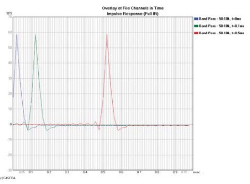
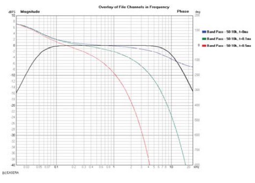
An increase in propagation delay — or any frequency independent delay, for that matter — increases the phase shift of a signal at the receiver location compared to when it originated (Fig. 1). The same device was measured three different times with a different propagation delay for each measurement. This could have been due to different microphone location or different DSP latency. In this case, a different signal delay was applied to illustrate the point.
In each case the magnitude response is the same but the phase response is different. To understand this, look at Fig. 2, which shows the impulse response, in the time domain, of these same measurements. The progressively later arrival of each impulse (more propagation delay) causes more phase shift.
To see the inherent phase response of a DUT, you would like to be able to remove all of the propagation delay (red and green traces in Figs. 1 and 2) so that you are left with only the phase shift caused by the DUT itself (blue trace in Figs. 1 and 2). But exactly how much time compensation (receive delay) should be used?
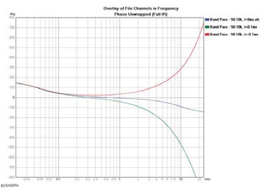
If you don’t remove all of the propagation delay, the phase response will continue to decrease, particularly in the high-frequency region. If you remove too much propagation delay, the phase response will increase, again predominantly in the high-frequency region. Both of these conditions are shown in Fig. 3.
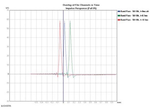
This latter condition indicates that energy came out of the DUT before it went into it. This is referred to as an acausal response, meaning that the output was not caused by the input. This is shown in Fig. 4 as the impulse arriving before time t = 0. This can’t happen in real time but can be made to appear as if it did with different analyzer settings or post-processing of the measurement data.
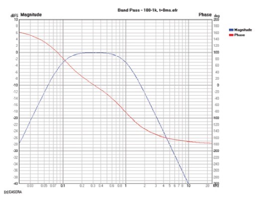
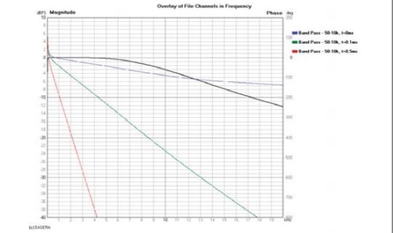
A loudspeaker can be modeled as a bandpass filter. At low frequency the magnitude response will be very low in level and increasing with increasing frequency until it reaches its passband level and flattens out. At a higher frequency the magnitude response will begin to decrease with increasing frequency (Fig. 5). The phase response for this DUT is also shown.
In this example, I selected a 1kHz corner frequency as the high-frequency limit to illustrate a concept detailed in a paper by Richard Heyser (1). This two-page paper is highly recommended reading. Its brevity greatly belies its substance.
Heyser stated that “If the value of time delay in the measuring medium is to be subtracted in the measurement process, as can be done for impulse, cross spectrum and TDS measurements, then the proper value of time delay has been subtracted, and the true acoustic position for the phase measurement has been obtained, when the plot of phase angle versus frequency approaches a flat horizontal line for frequencies well outside the pass band of the DUT.” In other words, you have removed the correct propagation delay when the phase response in the frequency region well above the cutoff frequency of the DUT approaches a horizontal line. This is exactly what is beginning to occur in Fig. 5 at approximately 8kHz and higher. The phase response is asymptotically approaching a horizontal line.
Notice also that in the higher-frequency region of the passband and just beyond (500 – 2,000Hz) the phase response is not flat. It is erroneous—albeit possible—to set a receive delay to yield a nearly horizontal phase response in this frequency region. This is a very common error and one that I formerly perpetrated with some regularity.
Now that you know what to look for in the phase response, how do you achieve it? You can look at Figs. 2 or 4 and conclude that the correct receive delay to apply is some time between the initial perturbation of the impulse response from a magnitude of 0 (or out of the noise floor) and its maximum value. You could iteratively try each incremental data point (sample) of the IR and look at the phase to see whether you had it right. This may become quite time consuming, however.
Alternatively, you can use group delay to help determine the correct receive delay. Group delay is defined as the negative rate of change of phase with respect to frequency.
τg = -dΦ/dω
In this equation the Greek letter omega (ω) denotes angular frequency which is simply 2π times frequency. The Greek letters tau (τ) and phi (Φ) denote group delay and phase, respectively. This is just a mathematical way of saying that the negative slope of the phase response gives the group delay response. This means that if the slope of the phase response is constant — i.e., a straight line — over a range of frequencies, then the group delay has a constant value over that same range of frequencies.
In real time the phase response always slopes down with increasing frequency. This means the slope is negative. If this actual slope is used as the group delay, it implies that group delay is negative; that is, the signal arrives at the mike/listener at some negative time (prior to when it left the loudspeaker). Because this can’t happen in real time, you negate the slope (multiply it by -1) of the phase response to get group delay. A negative slope times -1 will always yield a positive group delay (the signal arrives at the mike/listener at some time after it left the loudspeaker).
To see the constant slope of the phase response you must view it on a linear frequency scale. When viewed on the more common logarithmic frequency scale, the phase response appears to curve down more in the high frequency region. This is simply a result of viewing phase on a log frequency scale. The phase response curves of Fig. 1 are shown on a linear frequency scale in Fig. 6.
Here you see that progressively greater propagation delay results in a straight line (in the high-frequency region) with progressively greater downward slope (compare Fig. 6 with Fig. 2).
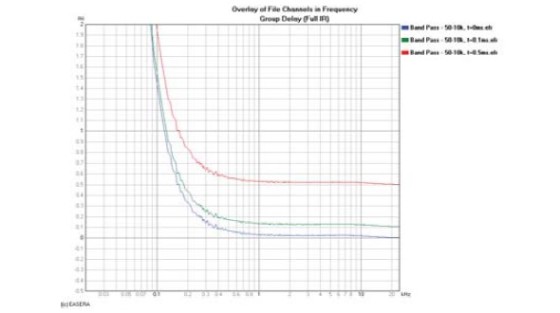
The group delay for these phase responses is shown in Fig. 7. The group delay in the very high-frequency region of each of these curves approaches the actual propagation delay for each measurement.
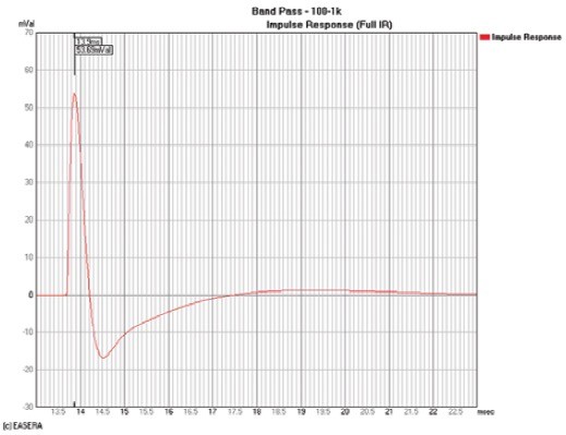
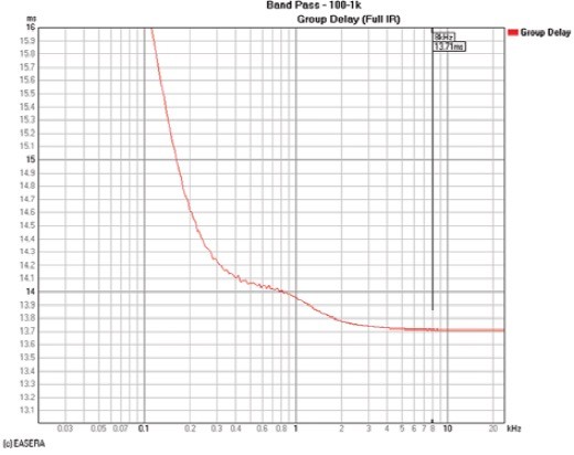
The example in Fig. 5 has a much lower cutoff frequency (high-frequency limit) than the example in Fig. 1. Because it has less high-frequency output and more phase shift as seen in the frequency domain, the impulse response (or the ETC) in the time domain will have a longer rise time. This makes it more difficult to determine its true propagation delay from these time domain graphs. The cursor in Fig. 8 shows the peak arrival at 13.9ms. However, the cursor at 8kHz on the group delay response shown in Fig. 9 indicates the propagation delay to be 13.71ms. This is the true propagation delay for this measurement.
If you had used 13.9ms as the receive delay, you would have removed 190